If two identical linear springs are connected symmetrically to a mass in a "V" shape, and an adjustable force is applied to the mass, when this force is varied, the resulting motion of the mass depends on the history of changes in the applied force under certain conditions . This phenomenon is called “hysteresis”. Hysteresis is usually found in electromagnetic systems, but this simple mechanical setup is also able of presenting hysteresis.
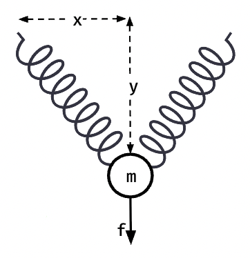
Describing the system
Describing the system
Hysteresis systems are not linear, however, we can analyze the forces acting on the mass as such:
F[y_]=f-2*k*y1-+
l
0
2
x
2
y
Where f is the sum of the external force acting on the mass and its weight, l0 is the natiral length of the spring, and k is the spring constant.
For this effect, there are two conditions:
For this effect, there are two conditions:
◼
l0<x: The springs are extended for y=0, and for every y. The forces have a sufficient upward component to balance the external force. There is only one equilibrium point.
◼
l0>x: The springs are compressed for y=0. They will be compressed for some y and extended for some others. There can be up to three equilibrium points. For this condition the phenomenon of hysteresis is observed.
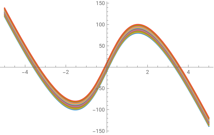
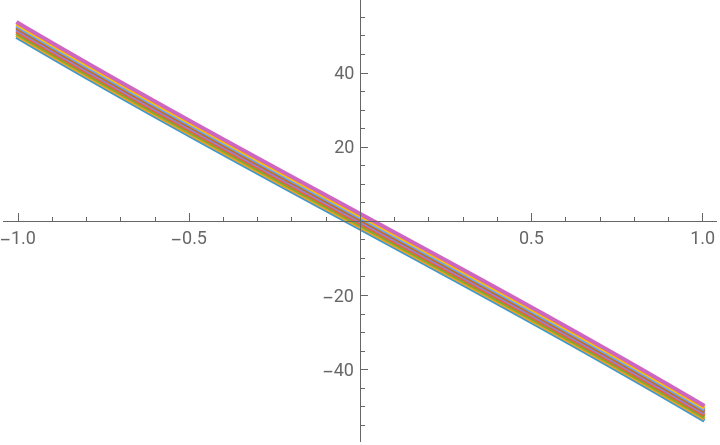
For some given values for f, k, x, l0 the graphs for the net force with respect to y can be created :
l0<x
l0<x
TableF[y_]=f-2*50*y1-+,{f,-1,1,0.5}
4
2
2
2
y
Out[]=
-1.-100y1-,-0.5-100y1-,0.-100y1-,0.5-100y1-,1.-100y1-
4
4+
2
y
4
4+
2
y
4
4+
2
y
4
4+
2
y
4
4+
2
y
In[]:=
Plot[Evaluate[Out[28]],{y,-5,5}]
Out[]=
l0<x
l0<x
TableF[y_]=f-2*50*y1-+,{f,-2,2,0.5}
2
2
4
2
y
Out[]=
-2.-100y1-,-1.5-100y1-,-1.-100y1-,-0.5-100y1-,0.-100y1-,0.5-100y1-,1.-100y1-,1.5-100y1-,2.-100y1-
2
16+
2
y
2
16+
2
y
2
16+
2
y
2
16+
2
y
2
16+
2
y
2
16+
2
y
2
16+
2
y
2
16+
2
y
2
16+
2
y
In[]:=
Plot[Evaluate[Out[60]],{y,-1,1}]
Out[]=
Critical Points
Critical Points
Now, if we solve F’(y)=0 we can find the critical points:
In[]:=
F[y_]=f-2*k*y1-+;F'[y]
l
0
2
x
2
y
Out[]=
--2k1-
2k
2
y
l
0
3/2
(25+)
2
y
l
0
25+
2
y
In[]:=
Solve[F'[y]==0,y,Reals]
Out[]=
y,y
Different natural lengths
Different natural lengths
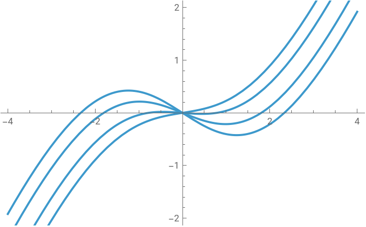
We can also make a graph for different values of l0, for an experiment with four different springs with different natural lengths:
In[]:=
ShowPlot2*y1-+,{y,-4,4},Plot2*y1-+,{y,-4,4},Plot2*y1-+,{y,-4,4},Plot2*y1-+,{y,-4,4}
3.8
2
3
2
y
3.5
2
3
2
y
3.1
2
3
2
y
2.8
2
3
2
y
Out[]=
Bibliography:[1] Mayergoyz, I. D. (2003). Mathematical models of hysteresis. IEEE Transactions on Magnetics, 22(5), 603–608. https://doi.org/10.1109/TMAG.1986.1064353
[2] Hysteresis in a simple V-shaped spring-mass system Christopher Ong Am. J. Phys. 89, 663–665 (2021). https://doi.org/10.1119/10.0003536
CITE THIS NOTEBOOK
CITE THIS NOTEBOOK
Hysteresis in a simple spring system
by Myrto Terpsiadou
Wolfram Community, STAFF PICKS, October 15, 2025
https://community.wolfram.com/groups/-/m/t/3560797
by Myrto Terpsiadou
Wolfram Community, STAFF PICKS, October 15, 2025
https://community.wolfram.com/groups/-/m/t/3560797