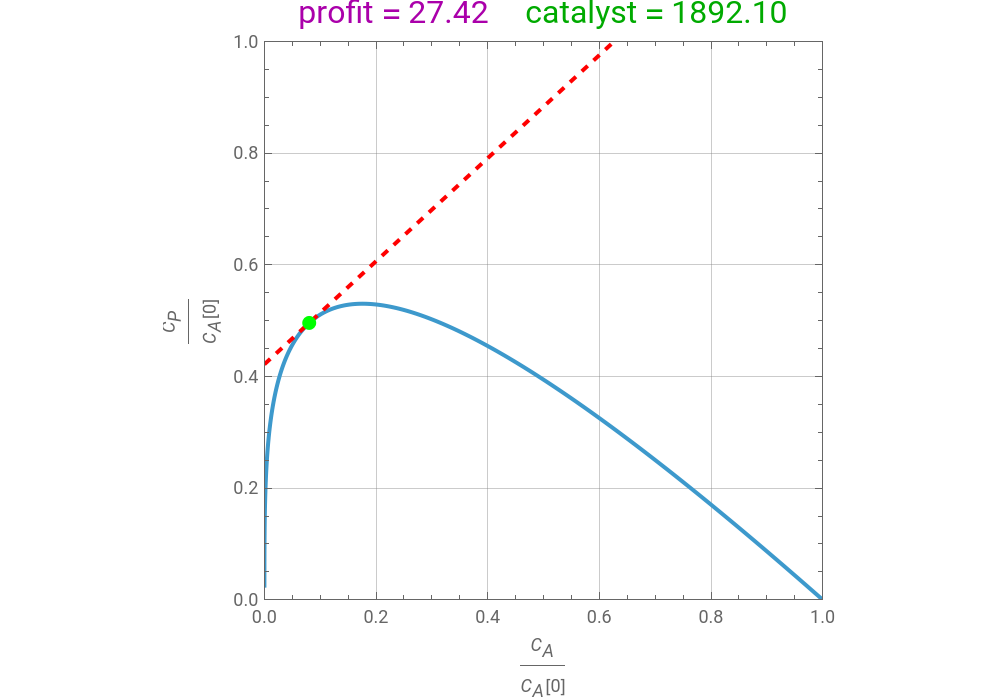
The synthesis of maleic anhydride, , involves the following reactions in the presence of a vanadium pentoxide catalyst:++2+2O (1)+3→4+O (2)+→6+3O (3)If air is present in excess, the concentration of oxygen can be considered as constant and the reaction rates are given by =, =, and =, where is the rate constant of reaction (expressed in kg catalyst), is the concentration of benzene, and is the concentration of maleic anhydride.The temperature-dependent rate constants are given by =4280, =70100, and =26.The governing equations at steady state, obtained by writing molar balances, for a packed-bed reactor modeled as a PFR (plug-flow reactor) are:=--, with (0)=10mol/ the concentration of benzene in the feed stream (i.e. at the entrance of the reactor), and=-, with (0)=0 the concentration of maleic anhydride in the feed stream, where =0.0025/s is the volumetric flow rate of the feed stream, which is composed mainly of air, and is the weight of catalyst (expressed in kg catalyst).The final/outlet concentrations of benzene () and maleic anhydride () are obtained by solving the steady-state equations numerically, with the weight of the catalyst ranging from 0 to 10,000 kg.This notebook plots the attainable region for maleic anhydride synthesis for a temperature equal to 600 K. A profit function is defined by , where and are user-set values of the prices of maleic anhydride and benzene. When this function is maximized, the optimal catalyst weight (shown in green) and the value (shown in magenta) are determined. The optimal outlet values of the concentrations of benzene () and maleic anhydride () are identified on the plot by the green dot. The dashed red line represents the equation =(α-β)/(0) and is always tangent to the attainable region.Attainable regions define the achievable compositions that may be obtained from a network of chemical reactions. The attainable region in composition space was first presented by Horn in 1964, with more recent extensions by Glasser and coworkers (1987).Reference:[1] F. J. M. Horn, “Attainable Regions in Chemical Reaction Technique,” Third European Symposium of Chemical Reaction Engineering, London: Pergamon Press, 1964.[2] D. Glasser, C. Crowe, and D. Hildebrandt, “A Geometric Approach to Steady Flow Reactors: The Attainable Region and Optimization in Concentration Space,” Industrial Engineering & Chemistry Research, 26(9), 1987 pp. 1803–1810.[3] W. D. Seider, J. D. Seader, and D. R. Lewin, Product and Process Design Principles: Synthesis, Analysis, and Evaluation, 2nd ed., New York: Wiley, 2004.
C
4
H
2
O
3
C
6
H
6
9
2
O
2
C
4
H
2
O
3
CO
2
H
2
C
4
H
2
O
3
O
2
CO
2
H
2
C
6
H
6
15
2
O
2
CO
2
H
2
r
1
k
1
C
A
r
2
k
2
C
P
r
3
k
3
C
A
k
i
i
3
m
-1
s
C
A
C
P
k
1
-12660
T
e
k
2
-15000
T
e
k
3
-10800
T
e
v
0
d
C
A
dW
k
1
C
A
k
3
C
A
C
A
3
m
v
0
d
C
P
dW
k
1
C
A
k
2
C
P
C
P
v
0
3
m
W
C
A
C
P
f(,)=(α-β)/(0)
C
P
C
A
C
P
C
A
C
A
α
β
f
max
C
A
C
P
f
max
C
P
C
A
C
A
In[]:=
T=600;(*temperature*)CostA=6;(*benzenecost=β *)CostP=6.5;(*maleicanhydridecost=α*)
In[]:=
v0=0.0025;cA0=10;k1=4280Exp;k2=70100Exp;k3=26Exp;
-12660
T
-15000
T
-10800
T
In[]:=
sol=NDSolve[{v0D[cA[W],{W,1}]-k1cA[W]-k3cA[W],cA[0]cA0,v0D[cP[W],{W,1}]k1cA[W]-k2cP[W],cP[0]0},{cA[W],cP[W]},{W,0,10000}];
In[]:=
obj[W_]:=First[Evaluate[CostPcP[W]-CostAcA[W]/.sol]];
In[]:=
solopt=NMaximize[{obj[W],W≥0},W];
In[]:=
plt1=ParametricPlot{cA[W]/cA0,cP[W]/cA0}/.sol,{W,0,10000},PlotRange{{0,1},{0,1}},ImageSize{500,350},PlotStyleThick,FrameLabel"[0]","[0]",PlotPoints1000,FrameTrue,GridLinesAutomatic,PlotLabelRow[{Style[Row[{"profit = ",NumberForm[solopt[[1]],{5,2}]}],Darker@Magenta,16]," ",Style[Row[{"catalyst = ",NumberForm[W/.solopt[[2]],{5,2}]}],Darker@Green,16]}];plt2=ParametricPlot[{x,(solopt[[1]]/10+CostAx)/CostP}/.sol,{x,0,1.0},PlotStyle{Thick,Red,Dashed},PlotRange{{0,1},{0,1}}];
C
A
C
A
C
P
C
A
In[]:=
Show[plt1,plt2,Graphics[{Green,PointSize[0.025],Point[{cA[W]/cA0,cP[W]/cA0}/.sol/.solopt[[2]]]}]]
Out[]=