This project is focused on the study of the graphs of possible positions for the chess endgames with three or less pieces on the board. The graphs are visualized as clearly as possible. An arbitrary size of the board is considered, although almost always only the 3x3 and 4x4 boards allow a convenient visualisation using the reduction modulo symmetries of the board. I also address the question of random walks on these graphs and the outcome of the game if the players make random moves. Also, at least a part of the graph has a natural layered structure based on the optimal game for the players. The graphs were separated into two parts, one of which is foliated in a natural way.
The endgame graphs
The endgame graphs
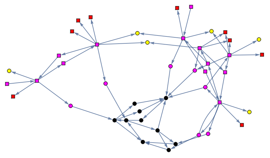
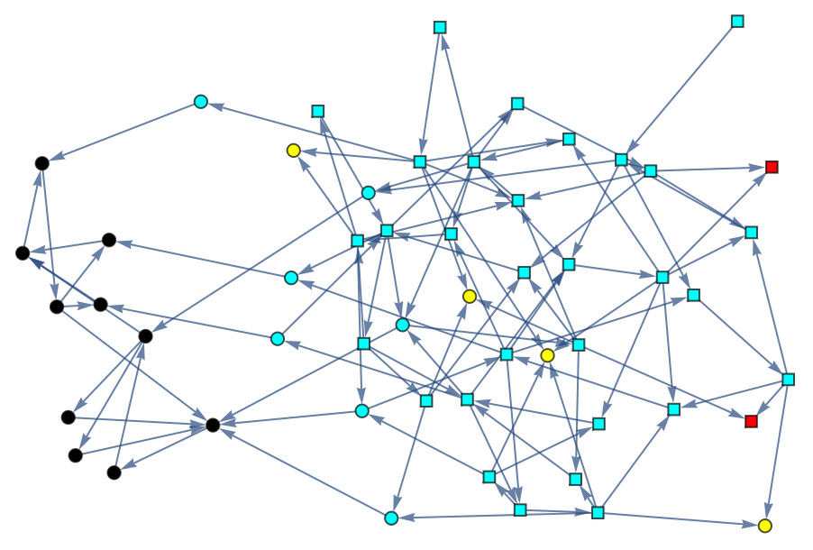
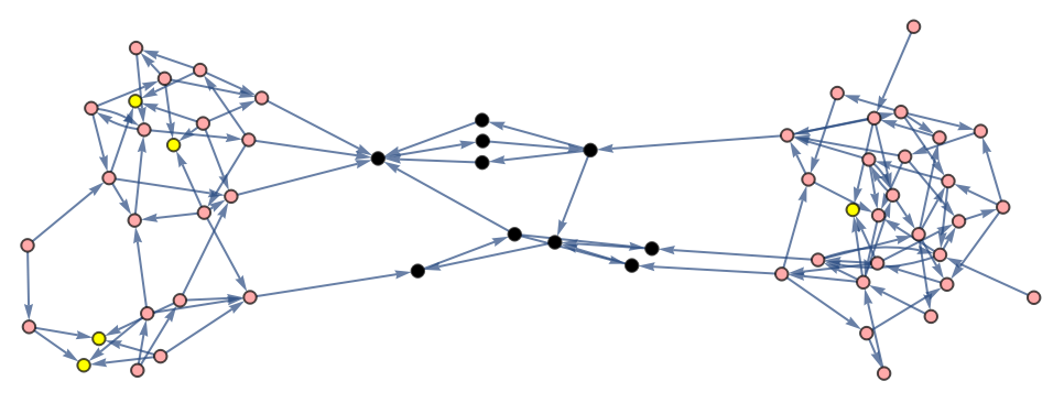
Let us start with the graphs of chess positions for separate pieces, including the positions with just two kings on the board (meaning the piece was captured). The piece is by default white. There are tooltips with positions to help the reader to explore the graphs. The white frame of the board means white is to move, and the black frame means it is black’s move. The graphs are factorized by the symmetry of the board, which reduces the number of nodes about eightfold, and makes the graphs readable. But it takes a bit more effort from the reader to keep track of moves, as two adjacent positions may be rotated and/or flipped in a different way. The shape of the vertices indicates the evaluation of the position, i.e. whether it is a win for white or a draw if the players play perfectly. Since black never has any pieces except king, a win for black is impossible. Also, we forget about the threefold repetition rule and the rule about 50 moves without a capture or a pawn move, because then the state of game should include the entire history of the game, and it will make the graphs far too complicated and unbearable to look upon.
In[]:=
showPieceGraph[3,"queen"]
Out[]=


In[]:=
showPieceGraph[3,"rook"]
Out[]=

In[]:=
showPieceGraph[3,"bishop"]
Out[]=

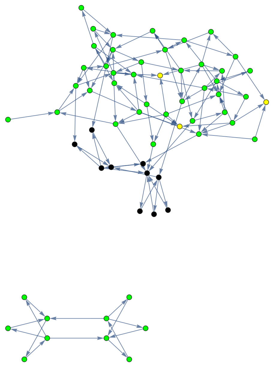
Notice how in the knight graphs a separate connected component emerges. The component consists of the positions with the knight in the middle of the board. He can never move, and he can never be captured, the two kings will just dance around him. In fact, it is isomorphic to the subgraph of the black vertices, i.e. the positions with two kings left on the board.
In[]:=
showPieceGraph[3,"knight"]
Out[]=

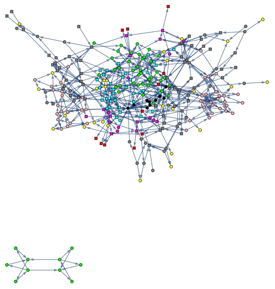
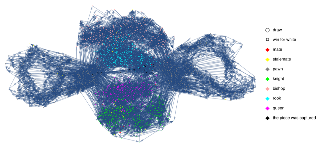
Now let's have a look at the positions with all possible pieces, including pawn. Since a pawn can be promoted to any piece, the pawn subgraph has edges going from it to subgraphs with other pieces. I considered the positions with the pawn on the first rank impossible. For the pawn positions, not all directions on the board are equivalent, since the pawn has to move in a specific direction, namely, up the board.
In[]:=
showGraph[3]
Out[]=

In[]:=
showGraph[4]
Out[]=
Random walks: per-node densities and the probability to win
Random walks: per-node densities and the probability to win
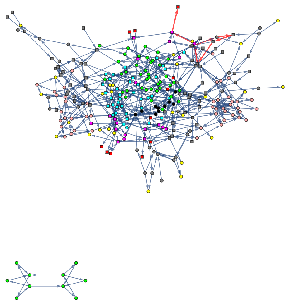
Take a random position with a pawn on the board. If the players make random moves starting from this position, they would essentially forming a random walk on the graph of all positions. The initial position is not exactly a random gray vertex, since different symmetry-reduced positions may have different degeneracy. The probability of a walk to start in a given pawn position is even before the symmetry reduction. In other words, the probability to start in a given vertex is proportional to its degeneracy. An example of a random walk is generated below:
In[]:=
graph=generateGraph[3];showWalk[graph,generateRandomWalk[3]]
Out[]=
Now let's ask the following question. Imagine a “gas of random walks”: each timestep the existing random walks take a random step forward, and another random walk is born. If some random walks hit the terminal states, like mate, stalemate or the capture of the piece, it disappears. In this model, what is the expected number of random walks in each node? Les us call the expected number of random walks density. We can answer the question in terms of probability flows. Each step, the density from each non-terminal vertex separates evenly and moves to the adjacent vertices. Also, due to the generation of a new random walk, it increases by a degeneracy of the vertex over total degeneracy of all vertices. The two sentences above are, in truth, a verbal description of a system of linear equations. By solving the system, one can find the densities of random walks in each vertex. In the graph below, the size of the vertex represents the density of walks in the log scale. The vertices in the connected component of a-knight-in-the-middle have zero size, because there is no way to achieve these positions starting with a pawn on the board.
(Almost) foliated graphs
(Almost) foliated graphs
How does one solve a game?
Let’s consider an example of tic-tac-toe game ( describes in detail in https://writings.stephenwolfram.com/2022/06/games-and-puzzles-as-multicomputational-systems/ ). The graph of the states of a tic-tac-toe game has a natural layered structure. The k-th layer consists of vertices with k moves made from the beginning of the game. We will describe a backtracking algorithm. First, we mark the terminal nodes, which are exactly vertices form the last layer, as wins, losses or draws, because it is clear for them. After that, we are able to evaluate the next-to-last layer of vertices. If it is first player to move, and there exists at least one edge to a vertex that is winning for the first player, we mark the position as winning for the first player. If all the edges lead to lost for the first player positions, then the vertex is marked as lost for the first player. If it was the second player to move, we would have a symmetric algorithm. It is clear that the algorithm visits every vertex in the graph, layer by layer.
Tic-tac-toe graph has a natural layered structure, because, by looking at a position, one can tell that the game will end in exactly k moves. Chess is fundamentally different from tic-tac-toe, because there is no natural way to assign a layer number to a position. The graph is not even acyclic, as the tic-tac-toe graph. If one tries to apply the backtracking algorithm to chess (starting with the mate, stalemate and two bare kings vertices as terminal states), the algorithm will not necessarily visit every vertex. But what if we do apply backtracking to chess? At the k-th step, the algorithm will visit the vertices such that they are either forced mates in k moves or forced draws in k moves. In case you wonder, forced draws are rarer, but they do exist. For example, here white is guaranteed to lose their knight in three half-moves if black makes reasonable moves. Black’s to move:
Let’s consider an example of tic-tac-toe game ( describes in detail in https://writings.stephenwolfram.com/2022/06/games-and-puzzles-as-multicomputational-systems/ ). The graph of the states of a tic-tac-toe game has a natural layered structure. The k-th layer consists of vertices with k moves made from the beginning of the game. We will describe a backtracking algorithm. First, we mark the terminal nodes, which are exactly vertices form the last layer, as wins, losses or draws, because it is clear for them. After that, we are able to evaluate the next-to-last layer of vertices. If it is first player to move, and there exists at least one edge to a vertex that is winning for the first player, we mark the position as winning for the first player. If all the edges lead to lost for the first player positions, then the vertex is marked as lost for the first player. If it was the second player to move, we would have a symmetric algorithm. It is clear that the algorithm visits every vertex in the graph, layer by layer.
Tic-tac-toe graph has a natural layered structure, because, by looking at a position, one can tell that the game will end in exactly k moves. Chess is fundamentally different from tic-tac-toe, because there is no natural way to assign a layer number to a position. The graph is not even acyclic, as the tic-tac-toe graph. If one tries to apply the backtracking algorithm to chess (starting with the mate, stalemate and two bare kings vertices as terminal states), the algorithm will not necessarily visit every vertex. But what if we do apply backtracking to chess? At the k-th step, the algorithm will visit the vertices such that they are either forced mates in k moves or forced draws in k moves. In case you wonder, forced draws are rarer, but they do exist. For example, here white is guaranteed to lose their knight in three half-moves if black makes reasonable moves. Black’s to move:
The backtracking will mark every winning position as winning. If a given position is winning, white can force a mate in k moves. All the positions with k=1 (and white’s to move) were marked as winning manually in the beginning. All the positions with k=2 (and white’s to move) would be also marked as winning as there is such move that it will lead to a position with black’s to move, and every black’s move leads to a position with k=1. Notice that the positions with black’s to move that are winning for white will also be marked as winning. After the backtracking visited every vertex it could, if there are unmarked vertices left, they have to be draws, so we can safely mark them as draws. Thus, the backtracking algorithm with a slight modification can solve games with acyclic graphs as well.
This allows us to introduce layers as vertices with forced termination in a certain number of half-moves. The foliation we get is a bit more complex than the classical foliation, since we can have vertices unvisited by the backtracking algorithm, namely, the positions such that it’s a draw by white’s inability to win, so the game will loop if white don’t want to get to drawn terminal states. I think it is reasonable to have a separate graph for such vertices when we represent a graph in the context of foliation. The first graph is a foliated graph of the positions “guaranteed mate in k moves if white plays rationally” or “guaranteed draw in k moves if black plays rationally”. The second graph contains the vertices unvisited by the backtracking algorithm, “draws by the white’s inability to win”.
Also, in the first graph I left the edges that go down the layers and not between positions evaluated differently, so they are perfect play edges by white in a winning subgraphs and perfect play edges by black in a drawn subgraph. In the second graph, all the edges are present except those edges that go to the positions from first graph, so they are perfect play edges by black.
This allows us to introduce layers as vertices with forced termination in a certain number of half-moves. The foliation we get is a bit more complex than the classical foliation, since we can have vertices unvisited by the backtracking algorithm, namely, the positions such that it’s a draw by white’s inability to win, so the game will loop if white don’t want to get to drawn terminal states. I think it is reasonable to have a separate graph for such vertices when we represent a graph in the context of foliation. The first graph is a foliated graph of the positions “guaranteed mate in k moves if white plays rationally” or “guaranteed draw in k moves if black plays rationally”. The second graph contains the vertices unvisited by the backtracking algorithm, “draws by the white’s inability to win”.
Also, in the first graph I left the edges that go down the layers and not between positions evaluated differently, so they are perfect play edges by white in a winning subgraphs and perfect play edges by black in a drawn subgraph. In the second graph, all the edges are present except those edges that go to the positions from first graph, so they are perfect play edges by black.
The graphs for separate pieces become simple enough to render the vertices as boards:
The graphs with rendered boards as vertices are divided into their weakly connected components for stylistic reasons.
Keywords
Keywords
◼
Graphs
◼
Chess
◼
Endgames
◼
Random walks
◼
Graph foliations
Acknowledgements
Acknowledgements
The author would like to thank Stephen Wolfram not only for suggesting the project, but also for convincing the author that the project is reasonable, because the author used to think that trying to visualize and structure the chess endgames graphs is a hopeless idea. The author also thanks his mentor, Connor Gray, for inspiring conversations and code reviews. Last, but not least, the author would like to thank Bradley Klee for encouraging the author to look for a way to foliate the graphs and for long fruitful conversations.
References
References
CITE THIS NOTEBOOK
CITE THIS NOTEBOOK
Multiway graphs for minimal chess endgames
by Pavel Arkhipov
Wolfram Community, STAFF PICKS, July 19, 2022
https://community.wolfram.com/groups/-/m/t/2575537
by Pavel Arkhipov
Wolfram Community, STAFF PICKS, July 19, 2022
https://community.wolfram.com/groups/-/m/t/2575537