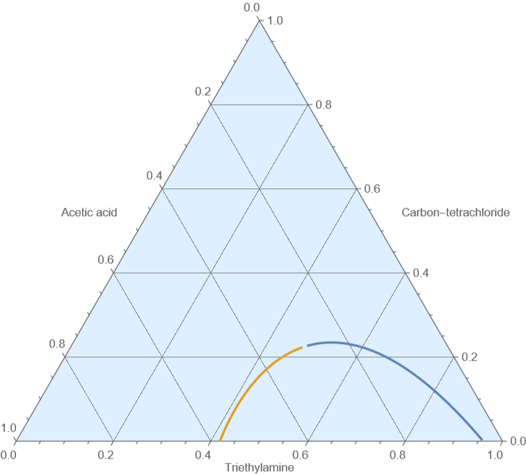
1- We compute the LLE diagram for Triethylamine (1) - Carbon-tetrachloride (2) - Acetic-acid (3) at 293 K and 1 atm
2- Feed is 10 mol% carbon tetrachloride (CCl4) and 90 mol% acetic acid (C2H4O2) with flow rate of 10.0 kmol/hr. Solvent is pure triethylamine (C6H15N). All streams and extraction equipment are at 293K and 1 bar. We solve for a two-stage crossflow system where the solvent flow rates are equal : S1 = S2 = 10 kmol/hr.
3- Feed is 40 mol% carbon tetrachloride (CCl4) and 60 mol% acetic acid (C2H4O2) with flow rate of 10.0 kmol/hr. Solvent is 10.0 kmol/hr of pure triethylamine (C6H15N). All streams and extraction equipment are at 293K and 1 bar. We consider a counter-current extractor in order to achieve a raffinate stream purity less than 4.89 mol% carbon tetrachloride. We find that three stages are sufficient.
Type I LLE ternary diagram for Triethylamine (1) - Carbon-tetrachloride (2) - Acetic-acid (3) at 293 K and 1 atm
Type I LLE ternary diagram for Triethylamine (1) - Carbon-tetrachloride (2) - Acetic-acid (3) at 293 K and 1 atm
Gas constant, temperature and binary interaction parameters for the NRTL model
In[]:=
param={a120.2,a130.2,a320.2,A120.,B12−303.24,A210.,B2190.396,A130.,B131162.9,A310.,B31−143.69,A230.,B23350.19,A320.,B3275.515};
In[]:=
TK=293.0;
Activities using the NRTL model
In[]:=
GAMMA1=Exp[(t21G21x2+t31G31x3)/(x1+G21x2+G31x3)+x1/(x1+G21x2+G31x3)(-(x2t21G21+x3t31G31)/(x1+G21x2+G31x3))+x2G12/(G12x1+x2+G32x3)(t12-(x1t12G12+x3t32G32)/(G12x1+x2+G32x3))+x3G13/(G13x1+G23x2+x3)(t13-(x1t13G13+x2t23G23)/(G13x1+G23x2+x3))]/.x31-x1-x2;GAMMA1p=Exp[(t21G21xp2+t31G31xp3)/(xp1+G21xp2+G31xp3)+xp1/(xp1+G21xp2+G31xp3)(-(xp2t21G21+xp3t31G31)/(xp1+G21xp2+G31xp3))+xp2G12/(G12xp1+xp2+G32xp3)(t12-(xp1t12G12+xp3t32G32)/(G12xp1+xp2+G32xp3))+xp3G13/(G13xp1+G23xp2+xp3)(t13-(xp1t13G13+xp2t23G23)/(G13xp1+G23xp2+xp3))]/.xp31-xp1-xp2;GAMMA2=Exp[(t12G12x1+t32G32x3)/(G12x1+x2+G32x3)+x1G21/(x1+G21x2+G31x3)(t21-(x2t21G21+x3t31G31)/(x1+G21x2+G31x3))+x2/(G12x1+x2+G32x3)(-(x1t12G12+x3t32G32)/(G12x1+x2+G32x3))+x3G23/(G13x1+G23x2+x3)(t23-(x1t13G13+x2t23G23)/(G13x1+G23x2+x3))]/.x31-x1-x2;GAMMA2p=Exp[(t12G12xp1+t32G32xp3)/(G12xp1+xp2+G32xp3)+xp1G21/(xp1+G21xp2+G31xp3)(t21-(xp2t21G21+xp3t31G31)/(xp1+G21xp2+G31xp3))+xp2/(G12xp1+xp2+G32xp3)(-(xp1t12G12+xp3t32G32)/(G12xp1+xp2+G32xp3))+xp3G23/(G13xp1+G23xp2+xp3)(t23-(xp1t13G13+xp2t23G23)/(G13xp1+G23xp2+xp3))]/.xp31-xp1-xp2;GAMMA3=Exp[(t13G13x1+t23G23x2)/(G13x1+G23x2+x3)+x1G31/(x1+G21x2+G31x3)(t31-(x2t21G21+x3t31G31)/(x1+G21x2+G31x3))+x2G32/(G12x1+x2+G32x3)(t32-(x1t12G12+x3t32G32)/(G12x1+x2+G32x3))+x3/(G13x1+G23x2+x3)(-(x1t13G13+x2t23G23)/(G13x1+G23x2+x3))]/.x31-x1-x2;GAMMA3p=Exp[(t13G13xp1+t23G23xp2)/(G13xp1+G23xp2+xp3)+xp1G31/(xp1+G21xp2+G31xp3)(t31-(xp2t21G21+xp3t31G31)/(xp1+G21xp2+G31xp3))+xp2G32/(G12xp1+xp2+G32xp3)(t32-(xp1t12G12+xp3t32G32)/(G12xp1+xp2+G32xp3))+xp3/(G13xp1+G23xp2+xp3)(-(xp1t13G13+xp2t23G23)/(G13xp1+G23xp2+xp3))]/.xp31-xp1-xp2;G12=Exp[-a12t12];G21=Exp[-a12t21];G13=Exp[-a13t13];G31=Exp[-a13t31];G32=Exp[-a32t32];G23=Exp[-a32t23];t13=A13+B13/TK;t23=A23+B23/TK;t12=A12+B12/TK;t32=A32+B32/TK;t31=A31+B31/TK;t21=A21+B21/TK;
In[]:=
K={GAMMA1/GAMMA1p,GAMMA2/GAMMA2p,GAMMA3/GAMMA3p}/.param;
In[]:=
z={0.6,0.2,0.2};
In[]:=
sol=FindRoot(K[[i]]-1)z[[i]](1+(K[[i]]-1)ϕ)0,x1z[[1]](1+(K[[1]]-1)ϕ),x2z[[2]](1+(K[[2]]-1)ϕ),xp1K[[1]]z[[1]](1+(K[[1]]-1)ϕ),xp2K[[2]]z[[2]](1+(K[[2]]-1)ϕ),{ϕ,0.1},{x1,0.9},{x2,0.1},{xp1,0.4},{xp2,0.001}
3
∑
i=1
Out[]=
{ϕ0.160537,x10.634579,x20.211183,xp10.419184,xp20.141525}
In[]:=
z={0.6,a,1-0.6-a}/.aa[s];eq1=(K[[i]]-1)z[[i]]/(1+(K[[i]]-1)ϕ)0/.x1x1[s]/.x2x2[s]/.xp1xp1[s]/.xp2xp2[s]/.ϕϕ[s];eq2=x1z[[1]]/(1+(K[[1]]-1)ϕ)/.x1x1[s]/.x2x2[s]/.xp1xp1[s]/.xp2xp2[s]/.ϕϕ[s];eq3=x2z[[2]]/(1+(K[[2]]-1)ϕ)/.x1x1[s]/.x2x2[s]/.xp1xp1[s]/.xp2xp2[s]/.ϕϕ[s];eq4=xp1K[[1]]z[[1]]/(1+(K[[1]]-1)ϕ)/.x1x1[s]/.x2x2[s]/.xp1xp1[s]/.xp2xp2[s]/.ϕϕ[s];eq5=xp2K[[2]]z[[2]]/(1+(K[[2]]-1)ϕ)/.x1x1[s]/.x2x2[s]/.xp1xp1[s]/.xp2xp2[s]/.ϕϕ[s];eq6=x1'[s]^2+x2'[s]^2+xp1'[s]^2+xp2'[s]^2+ϕ'[s]^2+a'[s]^21;derivinit={x1'[0]0,x2'[0]0,xp1'[0]0,xp2'[0]0,ϕ'[0]-1,a'[0]-0.001};init={x1[0](x1/.sol),x2[0](x2/.sol),xp1[0](xp1/.sol),xp2[0](xp2/.sol),ϕ[0](ϕ/.sol),a[0]0.6};system=Flatten[Join[{{eq1,eq2,eq3,eq4,eq5,eq6},derivinit,init}]];
3
∑
i=1
In[]:=
SOL=Quiet@NDSolve[system,{x1,x2,xp1,xp2,ϕ,a},{s,-10,10},AccuracyGoal->10]
Out[]=
x1InterpolatingFunction,x2InterpolatingFunction,xp1InterpolatingFunction,xp2InterpolatingFunction,ϕInterpolatingFunction,aInterpolatingFunction


In[]:=
upbound=SOL[[1]][[1]][[2]][[1]][[1]][[2]]lobound=SOL[[1]][[1]][[2]][[1]][[1]][[1]]
Out[]=
10.
Out[]=
-2.77547
In[]:=
DATA1=Table[{x1[s],x2[s],1-x1[s]-x2[s]}/.SOL,{s,lobound,upbound,0.01}];DATA2=Table[{xp1[s],xp2[s],1-xp1[s]-xp2[s]}/.SOL,{s,lobound,upbound,0.01}];
In[]:=
p0=TernaryListPlot[{Flatten[DATA1,1],Flatten[DATA2,1]},Joined->True,PlotStyle->Thick,GridLines->Automatic,FrameLabel->{"Triethylamine","Carbon-tetrachloride","Acetic acid"},PlotRange->All,Method->{"Backdrop"LightBlue}]
Out[]=
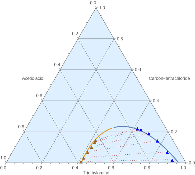
Tie Lines for Triethylamine (1) + Carbon-tetrachloride (2) + Acetic-acid (3) at 293 K and 1 atm obtained from Sorensen and Arlt, 1980
In[]:=
dataexp={{0.914,0.020,0.066,0.412,0.0090,0.579},{0.861,0.0710,0.068,0.414,0.034,0.552},{0.770,0.144,0.086,0.418,0.071,0.511},{0.698,0.192,0.110,0.423,0.104,0.473},{0.642,0.216,0.142,0.425,0.135,0.440},{0.62,0.222,0.158,0.425,0.147,0.428}}
Out[]=
{{0.914,0.02,0.066,0.412,0.009,0.579},{0.861,0.071,0.068,0.414,0.034,0.552},{0.77,0.144,0.086,0.418,0.071,0.511},{0.698,0.192,0.11,0.423,0.104,0.473},{0.642,0.216,0.142,0.425,0.135,0.44},{0.62,0.222,0.158,0.425,0.147,0.428}}
In[]:=
Pt={{2,1},{0,Sqrt[3.]}}/2;
In[]:=
data1=Table[Pt.{dataexp[[i]][[1]],dataexp[[i]][[2]]},{i,1,Length[dataexp]}]
Out[]=
{{0.924,0.0173205},{0.8965,0.0614878},{0.842,0.124708},{0.794,0.166277},{0.75,0.187061},{0.731,0.192258}}
In[]:=
data2=Table[Pt.{dataexp[[i]][[4]],dataexp[[i]][[5]]},{i,1,Length[dataexp]}]
Out[]=
{{0.4165,0.00779423},{0.431,0.0294449},{0.4535,0.0614878},{0.475,0.0900666},{0.4925,0.116913},{0.4985,0.127306}}
In[]:=
pexp=ListPlot[{data1,data2},PlotMarkers{Style["▲",Blue,14],Style["▲",Brown,14]}];
In[]:=
p=Show[p0,pexp,Graphics[{Darker@Red,Dotted,Table[Line[{data1[[i]],data2[[i]]}],{i,1,6}]}]]
Out[]=
In[]:=
p=Show[p0,Graphics[{Darker@Red,Dotted,Table[Line[{data1[[i]],data2[[i]]}],{i,1,6}]}]];
Cross-flow extractor
In[]:=
tbl1=Flatten[Table[{x1[s],x2[s]}/.SOL,{s,-2,1,0.0001}],1];
In[]:=
tbl2=Flatten[Table[{xp1[s],xp2[s]}/.SOL,{s,-2,3,0.001}],1];
In[]:=
rafnt=Evaluate[Interpolation[tbl2,InterpolationOrder1]]
Out[]=
InterpolatingFunction

In[]:=
Extrc=Evaluate[Interpolation[tbl1,InterpolationOrder1]]
Out[]=
InterpolatingFunction

Using interpolation to get tie lines
STAGE 1
STAGE 1
Feed and Solvent
Mixing Point
Extract and Raffinate Product
Plotting the first stage on the ternary diagram
STAGE 2
STAGE 2
Mixing Point
Extract and Raffinate Product
Plotting the first stage on the ternary diagram
Counter-current extractor
Counter-current extractor
Feed and Solvent
Mixing Point
Operating Point
Operating Point
Plotting Feed, Solvent, Extract, Raffinate and Operating Point
Stepping off Stages
Stepping off Stages
References
References
◼
[1] H. Binous and A. Bellagi, Calculation of Ternary Liquid - Liquid Equilibrium Data using Arc - Length Continuation, Engineering Reports, 3 (2), 2021.
◼
[2] J. M. Sorenson and W. Arlt, Liquid-Liquid Equilibrium Data Collection, Binary Systems, vol. V, part 1, 1979, Ternary Systems, vol. V, part 2, 1980, Ternary and Quaternary Systems, vol. 5, part 3, 1980, DECHEMA, Frankfurt (Main), Germany.
CITE THIS NOTEBOOK
CITE THIS NOTEBOOK
Liquid-liquid equilibrium curve and extraction for the ternary system
by Housam Binous & Ahmed Bellagi
Wolfram Community, STAFF PICKS, May 13, 2025
https://community.wolfram.com/groups/-/m/t/3459296
by Housam Binous & Ahmed Bellagi
Wolfram Community, STAFF PICKS, May 13, 2025
https://community.wolfram.com/groups/-/m/t/3459296