On the Stability Limit of Leapfrog Methods
On the Stability Limit of Leapfrog Methods


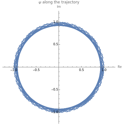
We study two leapfrog algorithms by applying them to the simple ordinary differential equation ψ(t)=-iωψ(t) with the initial value . The exact solution obviously is for all real and thus represents a rotation with angular velocity . In our context the significance of this equation is that it is the most general Schrödinger equation in a one-dimensional Hilbert space. Spectral decomposition allows any Schrödinger equation in a finite-dimensional Hilbert space to reduce to a finite set of copies of this case. The numerical solutions under consideration work in a two-dimensional Hilbert space formed by pairs , where the second component is defined to have the initial value . In this two-dimensional Hilbert space a time-stepping evolution algorithm is given in terms of a step matrix that in this case is a complex 2×2-matrix, the matrix elements of which are specified functions of the time step . In our case we have:
t
ψ(0)=
ψ
0
ψ(t)=exp(-iωt)
ψ
0
t
ω
(ψ(t),ϕ(t))
ϕ(0)=-iωψ(0)
h
ψ(t+h) |
ϕ(t+h) |
1- 2 τ 2 | τ- 3 τ 4 |
-τ | 1- 2 τ 2 |
ψ(t) |
ϕ(t) |
ψ(t+h) |
ϕ(t+h) |
1-iτ- 2 τ 2 | - 3 τ 8 |
-2τ | 1+iτ- 2 τ 2 |
ψ(t) |
ϕ(t) |
where . Here, as always in quantum theory, the angular velocity of phase rotation is associated with an energy . In the Demonstration code we use the numerical values . The Demonstration lets you visualize the complex quantities and for a discrete trajectory. Such a trajectory is defined by a number of rotation periods and a number of steps per rotation period. You can set both numbers using the sliders; also noninteger values make sense. For less than steps per period one sees singularities for and . Selecting the mode "eigenvalues" shows that then one of these eigenvalues of the step matrix has a modulus larger than 1. The quantities and vanish for the exact solution due to unitarity and energy conservation. They do not vanish exactly for the discrete trajectories defined by the two leapfrog algorithms. They can be inspected under the method "errors". The reason for considering these error measures is that they can also be computed in cases where the exact solution is not available.
τ=ωh
ω
ℏω
ω==ℏ=1
ψ
0
ψ
ϕ
π
ψ
ϕ
ν(t)=〈ψ(t)|ψ(t)〉-〈ψ(0)|ψ(0)〉
ϵ(t)=〈ψ(t)|ϕ(t)〉-〈ψ(0)|ϕ(0)〉
To put our main finding into perspective we notice that having steps per period should be compared with "sampling at Nyquist frequency", which is two steps per period. In engineering language we have to "oversample" by a factor to get a stable trajectory. As we can learn from this Demonstration, a much stronger oversampling is needed to get a trajectory that is moderately accurate.
π
π/2≈1.57
Details
Details
Snapshot 1: for only a few steps per rotation the trajectory is polygonal; the corresponding graphics for method sv give a more oblate, less circular trajectory
Snapshot 2: error curves for the same trajectory as snapshot 1
Snapshot 3: many steps per period create smooth error curves and trajectories
Snapshot 4: eigenvalues of the step matrix for a stable trajectory
Snapshot 5: eigenvalues of the step matrix for an exploding trajectory
This Demonstration builds trajectories by iterated application of the step matrix on states, starting from some initial state. In the present simple case, however, it is also possible to compute the generic power of the step matrix as a symbolic expression. For the Störmer–Verlet method this was done in[1, 2].
th
n
For the densified asynchronous leapfrog method, corresponding results follow from the fact that the step matrices and of the two methods, as given explicitly earlier, satisfy =M with the invertible matrix . In particular, the eigenvalues of the step matrices are the same. Let us collect the main formulas that hold for :
U
sv
U
dalf
U
dalf
-1
M
U
sv
M=
2 | - |
0 | 1 |
hω<2
n
U
sv
cos(nα) | βsin(nα) |
-1 β | cos(nα) |
α=2arctan
γ
β
β=1-
2
γ
γ=
ωh
2
For the error functions and (for =1) this implies
ν
ϵ
ψ
0
ν
sv
2
γ
2
sin(nα)
ϵ
sv
1
2
2
γ
The similarity of the step matrices by matrix implies the relations of the error functions for the two integration methods:
M
ν
dalf
2
γ
β
ν
sv
ϵ
dalf
1
2
ϵ
sv
-2
γ
ν
sv
As carried out in[1, 2], all these equations remain valid when the real number is replaced by the Hamiltonian operator and the definition of the and functions is understood as implying the scalar products with respect to the initial state of a trajectory. If you want to see the reasons behind the particular step matrices, inspect the code that defines them as a product of simple building blocks in accordance with the basic leapfrog idea.
ω
ν
ϵ
References
References
[1] U. Mutze, "The Direct Midpoint Method as a Quantum Mechanical Integrator." http://www.ma.utexas.edu/mp_arc/c/06/06-356.pdf.
[2] U. Mutze, "The Direct Midpoint Method as a Quantum Mechanical Integrator II." http://www.ma.utexas.edu/mp_arc/c/07/07-176.pdf.
Permanent Citation
Permanent Citation
Ulrich Mutze
"On the Stability Limit of Leapfrog Methods"
http://demonstrations.wolfram.com/OnTheStabilityLimitOfLeapfrogMethods/
Wolfram Demonstrations Project
Published: September 7, 2011