For those new to Mathematica I offer something I wish I had done many years ago, elaborating more carefully how nesting works in Table[ ]. This notebook draws from an example from Page 61 of Programming with Mathematica - An Introduction by Paul Wellin https://doi.org/10.1007/978-1-4612-2322-1.
Paul Wellin’s Nested table example
Paul Wellin’s Nested table example
In[]:=
examp1=Table[i+j,{j,1,4},{i,1,3}]
Out[]=
{{2,3,4},{3,4,5},{4,5,6},{5,6,7}}
From this passage on page 61 of Paul Wellin’s excellent text: “When there is more than one iterator, their order is important, because the value of the outer iterator is varied for each value of the inner iterator. In the above example, for each value of j (the inner iterator), i was varied from 1 to 3, producing four lists, each a three-element list for each of the four values of j. If you reverse the iterator order, you will get an entirely different list .”
This is an illustration of how the English language under-performs when describing mathematics. There are two problems. One is how we define “inner” (and by reference, its contra-twin “outer”); the other is the term “list.”
Beginning with the first problem, what does it mean to be “inner”? Here is a more general definition (note the most general would properly put “outer” beyond the edge of your screen or on your forehead or to the edge of the known universe, but that is another story). The problem is that “outer”, in the 2D circle example below and in the two iteration Table code can, for different reasons, be either on the left or the right.
In[]:=
Graphics[{Circle[{0,0},.5],Circle[{0,0},1],Text["inner",{0,0}],Text["outer",{-.75,0}],Text["outer",{.75,0}]}]
Out[]=
The English words “inner” and “outer” represent adjectives intended to convey the concept of “placement” within the broader idea of “order.” In our examp1 code: Table[i+j,{j,1,4},{i,1,3}], it is clear from Wellin’s example that he means {j, 1, 4} to be “inner.” But if one takes the placement adjective to apply only to the two iterators, neither are “in” or “out.” You can only describe one as inner when there are an uneven number of iterators, thus {j,1,4} is only “inner” in Table[i+j+k,{k,1,4},{j,1,4},{i,1,3}], where i and k are both outer.
What we might say is that there are three parts to the Table[ ] code: Table[expression, outer iterator, inner iterator]. This would only be true if one assumes only two iterators. AND it assumes reading left-to-right draws one more “inside” the text. Don’t try that in Hebrew.
Then there is the matter of the word “list.” Is an iterator a “list”? In the literal sense it is, but because the components of Table are sensitive to the context of Table[ ], the iterators are a special kind of list allowing only so many elements and only elements of a certain kind.
Complicating the matter further, here is the Wolfram Documentation for a 2D table. Wellin refers to his j as “the inner iterator” which is in the same position as i in the Documentation below that the says”i” is “outermost.”
In[]:=

Out[]=

Under “Details” in the Documentation for Table one finds the cryptic comment “usesthestandardWolframLanguageiterationspecification” which sends one searching for that. The closest I got was a Tech Note under Tutorials named "Some General Notations and Conventions" which is on the Web here.
The matter could be even further confused by the fact that Mathematica has two functions, Outer[ ] and Inner[ ] which perform the formal matrix algebra computations associated with the concepts of Outer Product and Inner Product (and its special case, the Dot Product). We shall ignore these as unrelated for the present, leaving them to become confused about on their own at a later time.
Let’s agree that Table code involves two major components: The expression to be calculated and the iterators, regardless of their number or order. Then, (thanks to Romke Bontekoe) let’s represent our code as a Table nested within another Table. This provides explicit clarity about what is “inner” at the modest cost of a bit of extra typing.
Let’s agree that Table code involves two major components: The expression to be calculated and the iterators, regardless of their number or order. Then, (thanks to Romke Bontekoe) let’s represent our code as a Table nested within another Table. This provides explicit clarity about what is “inner” at the modest cost of a bit of extra typing.
In[]:=
examp2=Table[Table[i+j,{i,3}],{j,4}]
Out[]=
{{2,3,4},{3,4,5},{4,5,6},{5,6,7}}
Here, i and j are in the same order in the expression and in the separate iterators. It is easy to identify i as the “inner” iterator as it is literally within the outer Table function where j appears as the outer iterator.
Using Trace to watch the table being built
Using Trace to watch the table being built
Now let’s use Mathematica’ Trace function to explain the workings of Wellin’s code step by step. This is examp1, NOT the examp2 revision just above, which we take up later.
In[]:=
trTab1=Trace[Table[i+j,{j,1,4},{i,1,3}](*examp1*)]
Out[]=
{Table[i+j,{j,1,4},{i,1,3}],{{i,1},{j,1},1+1,2},{{i,2},{j,1},2+1,3},{{i,3},{j,1},3+1,4},{{i,1},{j,2},1+2,3},{{i,2},{j,2},2+2,4},{{i,3},{j,2},3+2,5},{{i,1},{j,3},1+3,4},{{i,2},{j,3},2+3,5},{{i,3},{j,3},3+3,6},{{i,1},{j,4},1+4,5},{{i,2},{j,4},2+4,6},{{i,3},{j,4},3+4,7},{{2,3,4},{3,4,5},{4,5,6},{5,6,7}}}
Checking our dimensions, there are fourteen steps.
In[]:=
Dimensions[trTab1]
Out[]=
{14}
The first step
The first step
The first element is our input code, where we state the problem
In[]:=
trTab1[[1]]
Out[]=
Table[i+j,{j,1,4},{i,1,3}]
Last step
Last step
The last is our result, where we display the answer
In[]:=
trTab1[[14]]
Out[]=
{{2,3,4},{3,4,5},{4,5,6},{5,6,7}}
There are 12 intervening steps (no surprise this arises from 4*3 which are the end points of each range of the iterators. Later we will learn that this produces a 4x3 matrix. And at that time we MAY gain some insight as to how and why Mathematica is able to completely ignore rows and columns as identifying parts of matrix algebra.
How to organize the 12 intervening steps? One at a time, in order.
How to organize the 12 intervening steps? One at a time, in order.
Step 2
Step 2
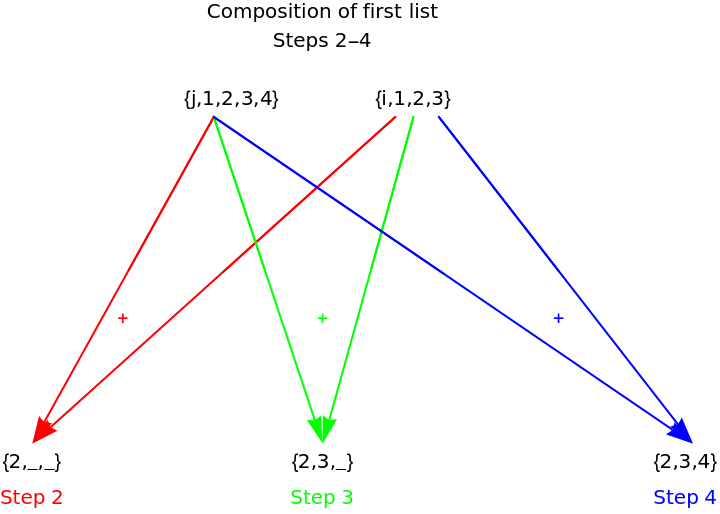
Step 2 takes the first element of each iterator list; it reads the first element, each, of i and j, adding them together because that is what the function requires. The addition is an artifact of the expression, the variables could be multiplied or one raised to a power of the other. A better way of seeing this list might be: {initial condition of i, initial condition of j, the expression, the result}.
In[]:=
trTab1[[2]]
Out[]=
{{i,1},{j,1},1+1,2}
In[]:=
{{i,1},{j,1},1+1,2}
Taking only the last element as our “solution” for this step, we have the first element in the first list of the final answer
In[]:=
trTab1[[2,4]]
Out[]=
2
Step 3
Step 3
Step 3 takes the second element of the outer list, i, but continues with the first element of the inner list, j, which will remain fixed until all the i elements are exhausted. The sum of these become the second element in the first list of our result.
In[]:=
trTab1[[3]]
Out[]=
{{i,2},{j,1},2+1,3}
In[]:=
{{i,2},{j,1},2+1,3}
Again, the last element from above, we have our "solution" for this step, the second element in the first list of the answer
In[]:=
trTab1[[3,4]]
Out[]=
3
Step 4 (completes the first list in the result)
Step 4 (completes the first list in the result)
Step 4 takes the third element of the outer list, i, but continues with the first element of the inner list, j. The sum of these become the third (and last) element in the first list of our result.
In[]:=
trTab1[[4]]
Out[]=
{{i,3},{j,1},3+1,4}
In[]:=
trTab1[[4,4]]
Out[]=
4
In[]:=
{{i,3},{j,1},3+1,4}
Our first list in our solution is now complete
In[]:=
examp1[[1]]
Out[]=
{2,3,4}
In[]:=
{trTab1[[2,4]],trTab1[[3,4]],trTab1[[4,4]]}
Out[]=
{2,3,4}
Or, a little shorter code mapping a pure function...
In[]:=
trTab1[[#,4]]&/@Range[2,4]
Out[]=
{2,3,4}
In[]:=
%==%==%
Out[]=
True
Graphically, here is where we are, having completed the first list in the solution
Out[]=
Step 5 (begins the second, of four, lists in the final solution)
Step 5 (begins the second, of four, lists in the final solution)
Having filled all the slots for i in the first list, j now begins with the second list. The first element of this list is the sum of the first element of i and the second element of j
In[]:=
{{i,1},{j,2},1+2,3}
Step 6
Step 6
{{i,2},{j,2},2+2,4}
Step 7 (last element in second list of output)
Step 7 (last element in second list of output)
{{i,3},{j,2},3+2,5}
The second list of our output is now
We are half-way finished. We have the first two of the four lists that j must create
Step 8 (first element in third list of output)
Step 8 (first element in third list of output)
How much more pedantry can you stand? We shall omit the narration in the coming steps, showing only the code as j cycles through i for a third time, first producing the first element in the third list of our output
{{i,1},{j,3},1+3,4}
Step 9
Step 9
{{i,2},{j,3},2+3,5}
Step 10
Step 10
{{i,3},{j,3},3+3,6}
Now 75% done, with three of the four lists needed for our output
Step 11
Step 11
Step 12
Step 12
Step 13
Step 13
Step 14 has our answer
Step 14 has our answer
Variations
Variations
Mathematica supplies a graphic showing all lists complete for examp1
Operations other than addition also work, merely following the same pattern
There are other ways to make nested lists
Notice that the first nested list may be displayed as a 4x3 matrix (using the “RC” convention of stating Rows first, followed by Columns). Mathematica does not care how you show it, to Mathematica it is still just a list of lists, whether organized in columns and rows or not...
...and the first elements of each row combine to make the first column, but Mathematica still does not care!!!
Is it possible that the most important lesson in all of this is that columns and rows are artifacts of human preference and historical teaching methodologies? That Mathematica ignores them is an important lesson. If Mathematica does not care then the math itself does not care and neither should we !!
Expanding Trace with the nested Table approach
Expanding Trace with the nested Table approach
Recall we had examp2 as a re-statement of examp1 in the form of nested tables.
Which got the same answer as we ponderously achieved in 12 steps above. For those with not enough tedium in their lives, Mathematica again rises to the occasion by tracing this explicit nesting.
Here, there are only 6 steps, with the first and last the same as in examp1, stating the problem and the final solution
But there are only four intervening steps, each having five dimensions, in each case the first stating the problem and the last providing an individual list of answers for that intervening step.
Each step is of the form...
...which, when the range of j is cycled through it, produces the same answer
Reverse entire i and j range lists
Reverse entire i and j range lists
Note below, when iterator lists are reversed we get three lists of four elements each, the transpose of our original answer.
The dimensions are reversed...
...as is the trace
Same 14 dimensions
Here are the intervening twelve steps between the first and last in a grid
Compare TreeForm of lists and elements in the first example with the same in the third example. Count the nodes in each.
The replication of the Trace on the nested Table method is left to the reader as an exercise, as the author is exhausted...