Idea
Idea
The project considers numerical modeling of quasi-conical quantum dots (QD) using the Wolfram Mathematica. Particular attention is paid to the study of the energy spectrum and wave functions of charge carriers in the presence of an impurity atom located in different regions of the QD. To solve the Schrödinger equation, analytical and numerical methods are used, including the use of special functions and numerical diagonalization of matrices. Calculations are performed for various geometric parameters and impurity positions, which allows us to estimate the influence of the shape, size and localization of the impurity center on the energy levels. The results obtained can be used in theoretical analysis and design of optoelectronic nanostructures with specified properties.
Constants
Constants
To begin, let’s introduce the parameters of the problem and the necessary physical constants that we will use
Free electron charge
e=;
Vacuum permittivity
In[]:=
ϵ0=;
Dielectric constant
In[]:=
ϵ=15.5;
Plank constant
In[]:=
ℏ=;
Free electron mass
In[]:=
m0=;
Electron effective mass in QD
μ=0.023*m0;
Bohr radius in QD
ab=15.5**10^-2(μ**10^3);
2
(1.054*)
-27
10
2
(4.803*)
-10
10
Converters to eV, meV and nm
In[]:=
ev=1.602*;mev=*ev;nm=;
-19
10
-3
10
-9
10
2D
QD Geometry for r = 10 and 60 Degree angle
a
B
Out[]=

In this problem we will consider an impurity inside such a QD, and we will try to theoretically and numerically describe this problem within the framework of the methods of Wolfram Language: According to Coulomb’s law, the impurity will interact with the electrons within the framework of the Coulomb interaction, the type of which is presented below.
Out[]=
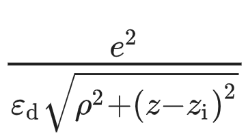
In the context of this problem, we will consider only two-dimensional interaction, therefore we discard the part responsible for axial interaction.
In[]:=
ClearAll[impurity2D];impurity2D[{x0_, y0_}][impurityQ_] := Block {c}, c = If[impurityQ, 1, 0]; *
1
mev * ab
c*
2
e
4*Pi * ϵ * ϵ0 * Sqrt[+]
2
(x-x0)
2
(y-y0)
Next, we need to solve the Schrödinger equation numerically in this system, taking into account that we have the following Hamiltonian of our problem
Out[]=
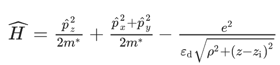
In[]:=
ClearAll[eigensystem2D];eigensystem2D[r_, α_][position_][impurityQ_] := Quiet @ NDEigensystem - * *(D[ψ[x, y], {x, 2}] + D[ψ[x, y], {y, 2}]) - impurity2D[position][impurityQ]*ψ[x, y] , DirichletCondition[ψ[x, y] 0, True] , ψ[x, y], {x, y} ∈ quasiCone2D[r, α], 10, Method "PDEDiscretization" {"FiniteElement", {"MeshOptions" {"MaxCellMeasure" 0.1, AccuracyGoal 2}}}
1
mev
2
ℏ
2 * μ *
2
ab
As you can see in this case we used the finite element method with special usage options (first 10 quantum states):
In[]:=
eigensystem2D[1,60][{0,0}][True]
Out[]=
{21.6145,49.8973,73.6653,87.4605,129.245,131.274,164.016,185.904,202.161,271.622},InterpolatingFunction[x,y],InterpolatingFunction[x,y],InterpolatingFunction[x,y],InterpolatingFunction[x,y],InterpolatingFunction[x,y],InterpolatingFunction[x,y],InterpolatingFunction[x,y],InterpolatingFunction[x,y],InterpolatingFunction[x,y],InterpolatingFunction[x,y]


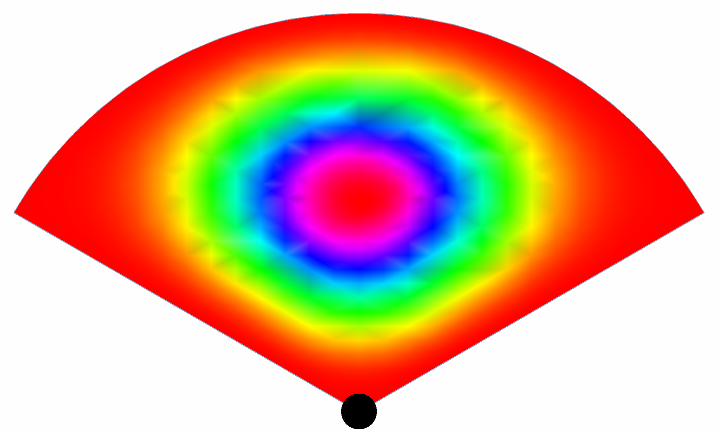
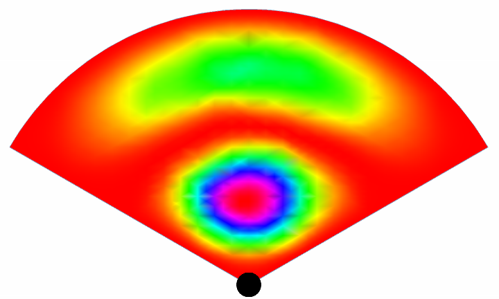
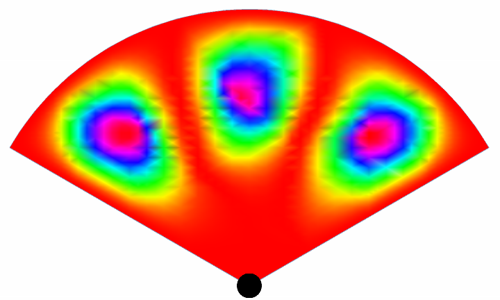
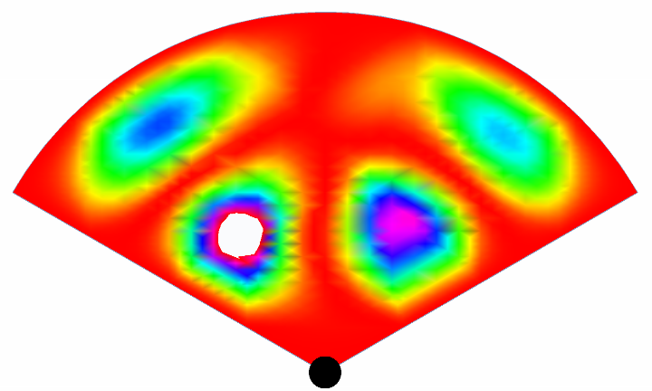
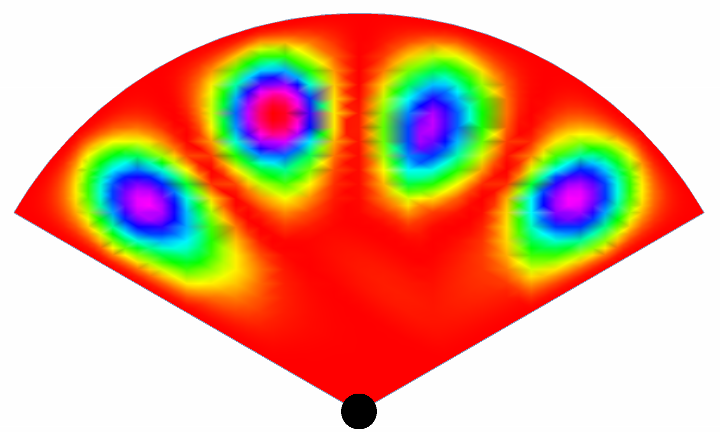
Let us consider the comparative behavior of the probability density of finding an electron in a QD based on the graphs below, for a relatively wide QD
Out[]=
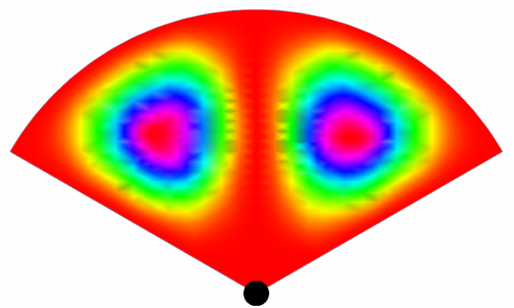
and a narrower and more elongated QD
Out[]=
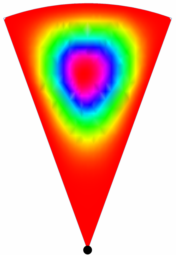
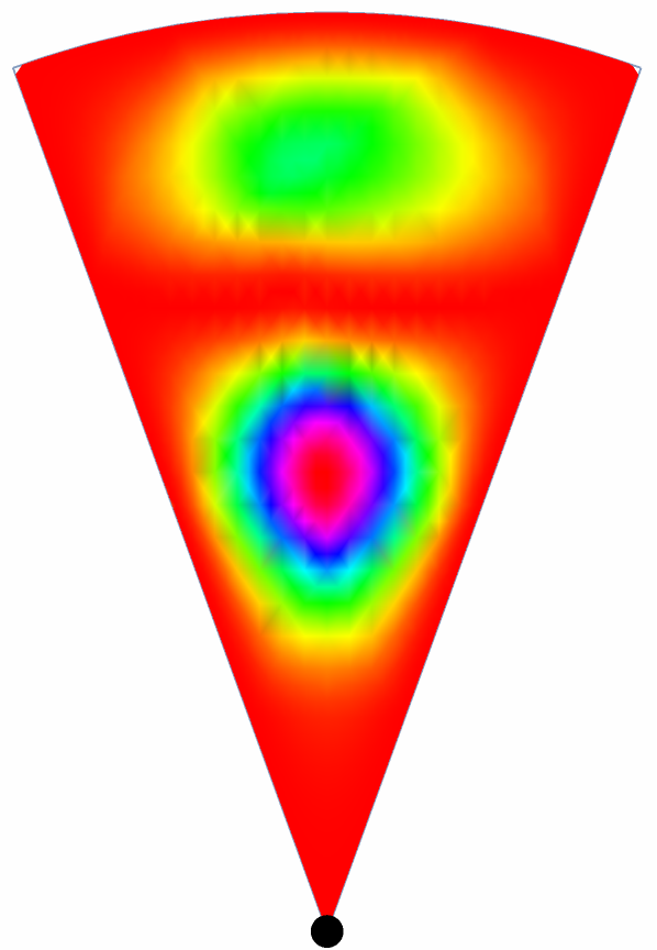
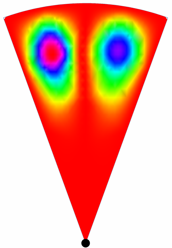
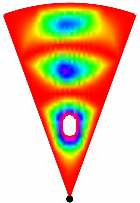
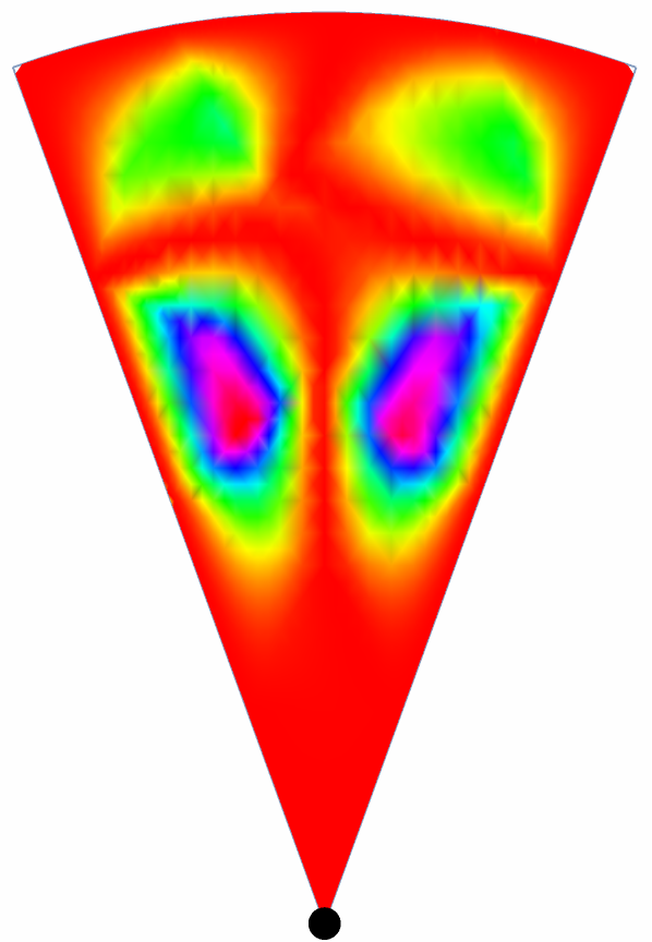
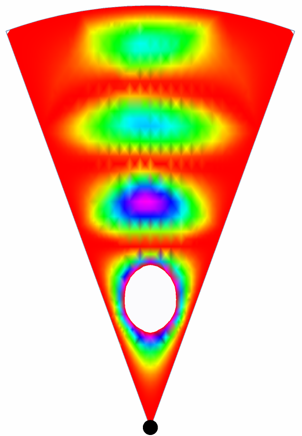
Based on the obtained results, many conclusions can be made regarding the optical and electronic properties of QDs, so below are presented the dependences of the system’s energy on its size, thereby showing what and how can be manipulated to obtain optimal results in a particular area of application:
And finally, the behavior of the binding energy is considered (the energy that must be communicated to the impurity in order to tear it away from the electron cloud)