Recently, an in-house model of OpenAI has cracked the 80-year-old Erdos conjecture in discrete math. Nature has featured this news in its recent issue, the Web has flooded with compelling animations (Alvaro Lozano Robledo, Vitaliy Kaurov, Anton Antonov 1, Anton Antonov 2) presenting the AI result in a form of magnificent graphs. This is certainly a right moment to support this rare surge of interest in fundamental math and graph theory by discussing the latter subject deeper giving tribute to other appealing concepts and results, even though they are not AI-generated.
This computational essay serves as a companion methods piece to the research article by Vasil A. Saroka
“On topologically frustrated polymers and where to find them”, Proc. A 2026; 482 (2339): 20250775. https://doi.org/10.1098/rspa.2025.0775
“On topologically frustrated polymers and where to find them”, Proc. A 2026; 482 (2339): 20250775. https://doi.org/10.1098/rspa.2025.0775
What is graph theory?
What is graph theory?
It is difficult to find a person who would not know that graph theory is something about points connected by lines - called graphs - a fancy geometry to represent data like social connections, to analyze computer grids or design neural networks. The basics go back to Leonard Euler and his problem of “Seven Bridges” of Königsberg, Fig. 1 (Euler1736). That problem was formalized in terms of “geometry of positions” referred to as geometria situs by Leibnitz and eventually solved by the polymath. While “Seven Bridges” has left a notable trace in field of graph theory, for example in terms of Eulerian paths in the graphs, it is, in fact, not a super hard problem and does not require a lot of efforts to understand that a walk passing through each line once requires less than two points that are connected to an odd number of other points. After all, any intermediate point of such a path must have an equal number of entries and exits, while initial and final points are allowed to have only one exit and one entry, respectively.
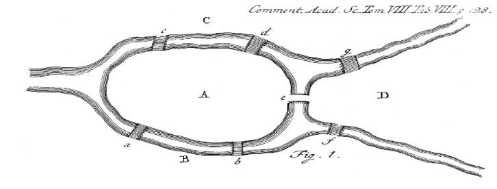
Figure 1. Seven Bridges of Königsberg: Leonhard Euler,“Solutio problematis ad geometriam situs pertinensis”, Commentarii Academiae Scientarum Imperialis Petropolitanae 8, 128–140 (1736)
This basic problem might give an impression that graph theory is about drawings and geometric configurations. Another extreme view point would be to consider graph theory as something purely arithmetic and algebraic. In this approach, one could associate each drawing with a matrix, reflecting connections between the points, the so-called adjacency matrix, which rows and columns represent the points of the graph and non-zero elements standing at the cross points of the rows and columns represent the connecting lines. The full stack of linear algebra operations is then applicable to our drawings. Both view points are valid and useful but as implied above there is something else. Specifically, the graph theory is capable of making statements about basic relations between the structural elements of our fancy geometrical creatures. This is where it is related to sets - a mathematical subject dealing with collections of elements of any nature in most general way. The progress in this side of graph theory was made from 30s to 60s, when a few fundamental theorems were proven. All these theorems deals with different aspects of our ability to partition a graph in terms of non-adjacent pairs of points - so-called matchings.
Matchings and non-Kekule radicals
Matchings and non-Kekule radicals
The concept of matchings is probably best explained in informal way. Similar to the Poincare’s theorem in topology, which has a laymen tangible Hairy ball theorem, the Hall’s theorem (Hall1935) in graph theory dealing with matchings has a statement captivating for any teenager - an ideal party making theorem. A good party shall involve boys and girls, but an ideal party shall make sure any of them have a familiar partner to support chat and dance. Such a perfect matching is possible if and only if any subgroup of boys combinedly knows more or equal number of girls. For a graph theory, however, matching sounds somewhat more boring. It is a regular subgraph of vertex degree one. If vertexes are the points constituting the graph, then the vertex degree is the number of lines, called also edges, connecting to a vertex. When the subgraph covers all the vertexes of the graph, then the matching is perfect. In some cases, such perfect matching is not achievable but the number of matching pairs is the largest possible for the given graph. Then the matching is called a maximum matching. There is one more possible situation. That is, when the given matching cannot be increased anymore but it is not the maximum matching for a graph in question. In this latter case, the matching is called a maximal matching. The Hall’s theorem gives a sufficient and necessary condition for the existence of a perfect matching in a bipartite graph, which consists of two internally disjoint sets of vertexes. The vertexes of the same disjoint set of a bipartite graph do not have lines connecting them, aptly reflecting the fact that boys and girls usually prefer to connect with the representatives of another group. However, “usually” does not mean “always” hinting that there may be more general situations. Likewise, in the graph theory, not always interesting graphs are bipartite. The perfect matching concept still applies though but the criterion for its existence is different from the one in Hall’s theorem. The necessary and sufficient condition for a perfect matching in a general graph was formulated by William Tutte in 1947 (Tutte1947). It is rather challenging to continue teenage party analogy at this point, but if we try to do so then the criterion states the following. If for any excluded subgroup of party participants the remaining party fell apart into friendly connected subgroups of even and odd size and the number of odd subgroups do not exceeds the number of excluded party participants, then the perfect party is possible. A fantastic relatation, isn’t it?
Matching are ubiquitous in various problems of practical use: from pair interactions in high-energy and condensed matter physics to network optimization in finances and computer sciences. Interestingly enough, they seem to appear in the organic chemistry earlier than anywhere else. At least, it can be tracked to the Kekule structure of benzene molecule, Fig. 2 (Kekule1866), that suggested a plausible cyclic configuration of single and double bonds between carbon atoms.
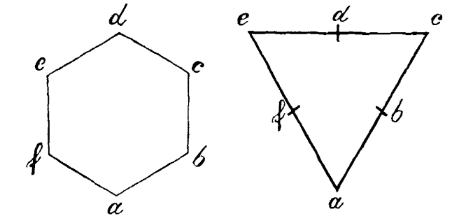
Figure 2. Ideally symmetric (left) and two atom grouped (right) presentations of a benzene molecule: August Kekulé, “Untersuchungen über aromatische Verbindungen”, Justus Liebigs Annalen der Chemie 137, 129–196 (1866)
In fact, if the carbon skeleton of a hydrocarbon molecule is a graph, then the double bonds are the matchings. In so-called conjugated molecules, where single and double bonds alternate maintaining the valency of 4 for each carbon atom, the breaking of this pattern yields an unpaired electron - radical. Radicals are chemically active. In addition they lead to paramagnetism due to the intrinsic angular momentum - spin - and associated magnetic moment of an electron. In the language of graph theory, an unpaired electron is a vertex that is left uncovered by a matching. Thus, matching patterns can be useful to detecting radicals and magnetism.
The peculiarities of magnetism are described by quantum mechanics. They go beyond graph theoretic considerations and require accurate accounting for the Coulomb and exchange interaction between electrons. For the simple case of a bipartite lattice, there are useful results along this way. The Lieb’s theorem (Lieb1989) and Ovchinnikov’s rule (Ovchinnikov1978) make a clear difference between radicals arising in the structures with and without so-called sublattice imbalance. The latter means the difference between the number of lattice sites in the two disjoint subsets of a bipartite lattice. The radical arising from the sublattice imbalance follow well-known for atoms Hund’s rule stating that an increasing number of unpaired electrons shall orient their spins in the same direction. For a small hydrocarbon with two free electrons, this means triplet state with a net spin S=1, while for the large molecules or crystals this results in the ferromagnetic ordering. The sublattice balanced radicals, however, break Hund’s rule, favoring orientation of spins in opposite directions. For the small hydrocarbon with two free electrons, this yields a singlet state S=0 with a net zero magnetic moment, while at a scale this is nothing else but a antiferromagnetic ordering. The natural question graph theory is capable to deal with is how radicals can arise in the sublattice balanced structures.
When is frustration topological?
When is frustration topological?
When a bipartite graph has a different number of vertices in the disjoint subsets, it is quite natural to expect that the perfect matching is not possible. However, such graphs may have an even total number of vertices, which make them less trivial than the most obvious case of a graph with an odd total number of vertices. In practice, there are some tricks which facilitate identification of such structures. All hydrocarbons, which are benzenoid molecules consisting from full hexagons, are based on honeycomb lattice, which has two major crystallographic directions dubbed zigzag and armchair. If one orients the graph of a benzenoid molecule such that zigzag direction is the horizontal one, then instead of counting vertices in the disjoint subsets, one can count only the vertices tracing the upper and lower boundary of the graph. The upper tracing vertices are called peaks, whereas lower ones are valleys. The difference between peaks and valleys is equal to the sublattice imbalance of the structure, which often also referred to as color excess (Sach1984, Cyvin1987, Cyvin1990). This allows us to quickly estimate if the given graph can host a Hund’s type radical and what shall be the total magnetic moment of the structure as per Lieb’s theorem and Ovchinnikov’s rule. The situation is furthest from trivial when we deal with a benzenoid molecule that has a zero sublattice imbalance. Peak and valleys approach fails here, while graph theory does not.
There are two ways to proceed with sublattice balanced structures: first principles analysis based on theorems and algorithmic approach. Here it is time to introduce the latter. For any bipartite graph, the maximum matching can be found by Hocroft-Karp-Karzanov algorithm (Hoprcoft1973, Karzanov1973). The number of vertices not covered by the maximum matching we shall call a graph deficit. The multiplicity of the radical is supplied by the deficit. It happens that for some structures deficit is non-zero even for sublattice balanced structures. This peculiar situation is called topological frustration (Wang2009). In fact, in the physics literature the sublattice imbalanced structures are also called topologically frustrated but labeled as class I, while sublattice balanced structures with a non-zero deficit are labeled as class II. However, graph-theoretically class II is more interesting as follows form the above discussion. In addition, class II is the one to which attention and topological considerations were drawn first (Gutman1974). Therefore, hereafter we take a freedom to allocate term topological frustration only to sublattice balanced graphs. The maximum matching search algorithms are useful for revealing radical nature of benzenoid hydrocarbons. Such algorithms provide a single footing for analysis of both sublattice balanced and imbalanced graphs.
Theorems and algorithms
Theorems and algorithms
The graph theory theorems are also a good supplement to algorithms. They provide an important conceptual framework for topological frustration analysis. The above-mentioned Tutte’s theorem implicitly introduces a set of special vertices, S, which can prevent a perfect matching in a graph. Let us restate this in a somewhat more mathematical language. If there is a set of vertices S for which the number of odd connected subgraphs, c(G-S), exceeds the number of vertices in the set |S|, then the perfect matching is not possible. In 1958 Claude Berge (Berge1958) extended this concept by introducing a formula linking it to the graph deficit. He found that the graph deficit is equal to the maximum of the difference between the number of odd connected subgraphs, obtained from the original graph by excluding the vertices S together with all incident edges, and the size of set S itself: max[c(G-S)-|S|]. The set S supplying this maximum is called a barrier in graph theory. Given a clear tendency to consider such effects as topological, as follows from introduction of the term “topological frustration”, we, however, prefer to call the peculiar S set an obstruction. In topology, an obstruction is something that separates equivalence classes distinguished by topological invariants. It is a barrier on the path of continuous transformation from one equivalence class to another. It seems that semantically graph theory barrier can be also dubbed a topological obstruction. In any case, what is really important here is that graph structure contains a special set of vertices. This set of vertices can be distinguished within the structure of a benzenoid hydrocarbon molecule and shed the light on the possible structural modifications that are allowed without affecting the deficit (Saroka2026). The revealed by theorems obstruction set of vertices in the graph allows one to modify the structure of the benzenoid hydrocarbon preserving its peculiar magnetic properties.
At last, we shall see how algorithms and theorems synergize together to reveal the full power of graph theory for the hydrocarbons analysis. Although the Tutte’s and Berge’s theorems reveal some structural elements of graphs such as an obstruction set, odd connected subgraphs and even connected subgraphs, this initial decomposition have that drawback that its elements are not uniquely defined. For example, as a rule, the obstruction set has many representations for a given graph. There may be multitude of them and they have a complex calculus so to say because the unions and intersections of obstruction sets are not always obstruction sets themselves. Mathematicians would say that the calculus of obstruction sets does not have a group structure. Not always this is a drawback but for the clarity of situation it would be useful to know some golden standard to start with. Then we would be able to decompose any graph into the above-mentioned structural elements with certainty and reveal their properties.
The golden standard is based on Gallai-Edmonds’ structural theorem (Gallai1964, Edmonds1965), which provides guidance on how to build a canonical obstruction set A. This allows one to identify two other sets, D and C, of odd and even subgraphs. In fact, the construction can start from D set, which is defined as a set of vertexes that are left uncovered by at least one maximum matching. Then the canonical obstruction set A is a set of vertices covered by every maximum matching and adjacent to at least one vertex of D set. The remaining vertexes of the graph belong to C set. To mine the D set from a graph with a brute force one may try to use maximum matching enumerating algorithm such as Uno’s algorithm (Bullard2014, Uno2001, Uno1997). This provides full information not only on the total number of maximum matchings but also on their full configurations which, from chemistry point of view, could be useful for resonance structure, Clar structure and aromaticity analysis. Generally speaking, such algorithms are slow and do not allow to find the answer in a polynomial time because the problem of counting matchings is #P-complete, which means it is at least as hard as NP problems (Valiant1979). In practice, this may not be as bad as it sounds, especially when dealing with simple graphs of benzenoid hydrocarbons. Yet, since we are only interested in structural decomposition, better approaches can be attempted. For example, one can use the following property of D set: the size of maximum matching in G graph is equal to the size of the maximum matching in G with any D vertex removed. Thus, any maximum matching algorithm can be used to dig the D set out. For a bipartite graph, the above-mentioned Hopcroft-Karp-Karzanov algorithm, as the most efficient one, may be a good work horse. In fact, it seems to be also under the hood of Uno’s algorithm for bipartite graphs (Uno1997). Using Hopcroft-Karp-Karzanov algorithm, all vertexes of the graph can be checked one by one by comparing the sizes of maximal matching for G with those for G without a given vertex. This requires to run algorithm at least the number of times equal to the number of vertexes in G. The most efficient way of decomposition, however, requires running a special maximum matching algorithm only once. This special algorithm is the blossom algorithm by Jack Edmonds (Edmonds1965). Its main power is that it can find maximum matchings in any graphs, including non-bipartite ones. However, its surprising side effect is that while finding a maximum matching it decomposes the graph into a forest of alternating trees. The vertices of such trees that are located at even distance from the tree root form D set, while vertices located at an odd distance form A set. The vertices of the graph that are not in the forest belong to C set. For a non-bipartite graph, the blossom algorithm has a special procedure of the graph reduction, which allows it to proceed with maximum matching search as if it would happen in a bipartite graph. For this, whenever it finds an odd cycle which is poetically called a flower, it shrinks such cycle into a single super vertex and restart the search on the new graph. Once the search is finished all the cycles can be unfolded (i.e. blossom as flowers) and the matching is revealed. Sometimes blossoming is happening several times and the maximum matching search looks like a summer meadow. Only vertices of D set can form flowers, therefore, in non-bipartite graphs the full D set includes D vertices of the mentioned alternating trees plus D vertices of flowers. To summarize, the blossom algorithm gives a direct access to the A and C sets, which can never be affected by the fading of flowers. The D set is then the remaining vertices of the graph.
By applying structural decomposition to a hydrocarbon molecule, one can get an insight about the origin of the radical properties. Combining this knowledge with Tutte’s and Berge’s theorems, one can assume what types of structural modifications will not affect the radical nature because extending any subgraph component with an even number of vertexes will not affect it parity. Of course, it is rather involved analysis and it would nice to have a programed implementation. Here, we present a simple interface developed in Wolfram Mathematica.
What are the options?
What are the options?
Mathematica has a build-in function
FindIndependentEdgeSet[]
that performs maximum matching search for any graph. As has been pointed out elsewhere, the details of such function implementation in Wolfram Language are not known but most likely it uses some variation of the blossom algorithm. The better variations include Blossom V by Kolmagorov (Kolmogorov2009) and Hopcroft-Karp-Karzanov generalization by Micali and Vazirani (Micali1980). In any case, there is no build-in implementation of the Gallai-Edmonds decomposition. Such code, however, is relatively easy to program adopting the second approach described above, which is implemented elsewhere:
In[]:=
maxMatchingSize[g_]:=Length[FindIndependentEdgeSet[g]]egDecomposition[g_]:=Module[{vertexList,max,d,a,c},vertexList=VertexList[g];max=maxMatchingSize[g];d=Select[vertexList,maxMatchingSize[VertexDelete[g,#]]==max&];a=Complement[AdjacencyList[g,Alternatives@@d],d];c=Complement[vertexList,d,a];<|"D"->d,"A"->a,"C"->c|>]
In[]:=
ResourceFunction["GallaiEdmondsDecomposition"][g]
The step-by-step demonstration of the blossom algorithm together with WL code can be also found as a Wolfram Demonstrations Project example contributed by Matthew Kusner, Stan Wagon.
Some details can also be found on the Blossom Algorithm page of Wolfram Math World. Such common sources as Wikipedia and Brilliant shall be also mentioned. Both contain nice pictures introducing the basic concepts of this algorithm such as stem, base, flower and etc. Pseudo codes with different degree of clarity and details can be found there. In terms of interactive examples, the project of Technische Universität München can be of great usefulness for understanding blossom algorithm step-by-step. Less useful, yet very appealing at the start can be some YouTube videos.
All in all, an efficient ready to use solution for the Gallai-Edmonds decomposition seems not to be available, let along its seamless integration for hydrocarbon analysis. Since we started with the recent advances in AI, it would be natural to suggest asking some AI model to “vibe code” an app with required functionality. We, however, did not outsource the pleasure of learning and developed this app from scratch. Therefore, before demonstrating the app use cases, we proceed with some technicalities that may be useful to know for those who wants to put hand on blossom algorithm for the first time. These technical details are not needed for using our Wolfram Language app and they can be safely skipped by those who want to jump straight into hydrocarbon analysis.
On the way to blossom
On the way to blossom
For some reason, all the tutorials on blossom algorithm implies that a reader is familiar with the graph scanning methods such as breadth first search. Along with depth first search, breadth first method is one of the basic in the graph theory. It allows to build a tree that spans the graph. Here it is worth reminding that a tree is a graph that lacks any cycles. That is why, building spanning trees is very useful for simplifying analysis of the complex graphs. Breadth first search has that property that it preserves the distances between the vertices, i.e. the distance between two points in the tree has the same length as in the original graph. Such an algorithm is implemented in WL:
BreadthFirstScan[g,vrt]
However, its essence can be also coded from scratch:
In[]:=
Clear[BFS];BFS[vidx_,graph_]:=Block[{Q,color,dist,parent,uidx},color=Table[0,{i,Length[graph]}];parent=Table[-1,{i,Length[graph]}];Q={};color[[vidx]]=1;AppendTo[Q,vidx];While[Q=!={},uidx=First@Q;Q=Rest@Q;(*scanovernearest-neighborsofthevertex*)Do[If[color[[i]]==0,color[[i]]=1;AppendTo[Q,i];parent[[i]]=uidx](*endIf*),{i,graph[[uidx]]}](*endDo*)](*endWhileQisnotempty*);Return[{vidx,color,parent}]](*endBlock*);
This code reveals the basic structures that can be used for the graph presentation. The color list is is used to track visited vertices. The position of the element denote the vertex number, while the value of the element equal to 0 or 1 denotes the visited and unvisited vertex, respectively. The parent list is used to store the spanning tree data. The length of this list is equal to the number of vertices in the graph. The position of the element corresponds again to the number of the vertex in the graph. The value of the element denotes the number of the parent vertex for this one. The root vertex is the only one that does not have a parent, therefore, it is marked by -1. The algorithm uses an abstract data structure called queue. It is implemented as the Q variable with the key queue property “first in - first out”. Since the scan runs over the nearest neighbors in the above function, the graph structure shall be given to it as a list, wherein element positions denote the vertices and the values of the element represent the list of neighbors. The function also needs an initial vertex number vidx to start scan with.
To test the above BFS[...] function, let us take the following graph, Fig. 3:
In[]:=
graph={{1,2,3},{3,4,5},{4,6},{2,6},{1},{3,3}};gedges=Flatten[Table[i#&/@graph[[i]],{i,Length[graph]}]];Graph[gedges,VertexLabels->Automatic]
Out[]=
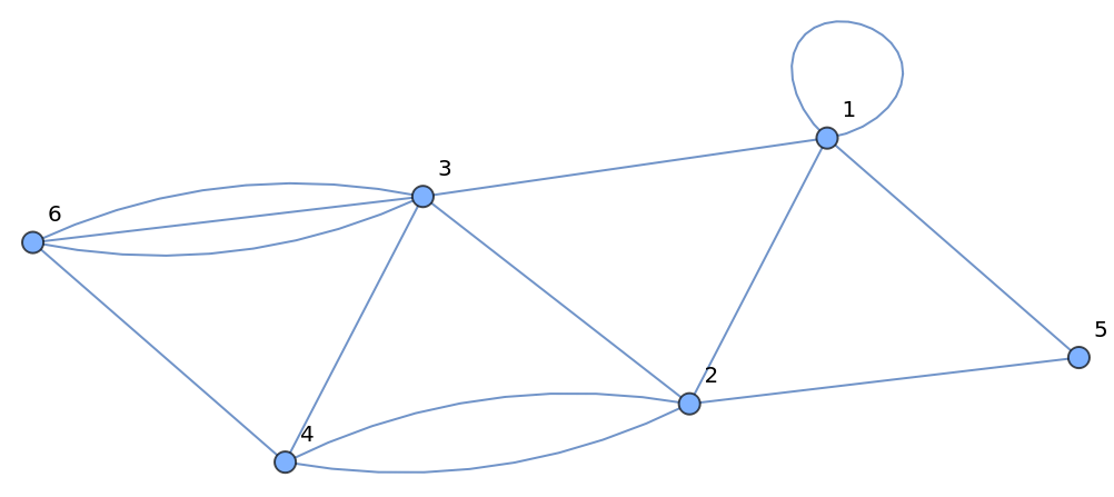
Figure 3. A graph to test BFS function
and run our function from vertex no. 1 to find a spanning tree:
In[]:=
root=1;d=BFS[root,graph]
Out[]=
{1,{1,1,1,1,1,1},{-1,1,1,2,2,3}}
The obtained output can be visualized, Fig. 4:
In[]:=
parent=d[[-1]];bfstree=DeleteCases[Table[If[parent[[i]]!=-1,iparent[[i]],Null],{i,Length[parent]}],Null];HighlightGraph[Graph[gedges,VertexLabels->Automatic],{bfstree,root}]
Out[]=
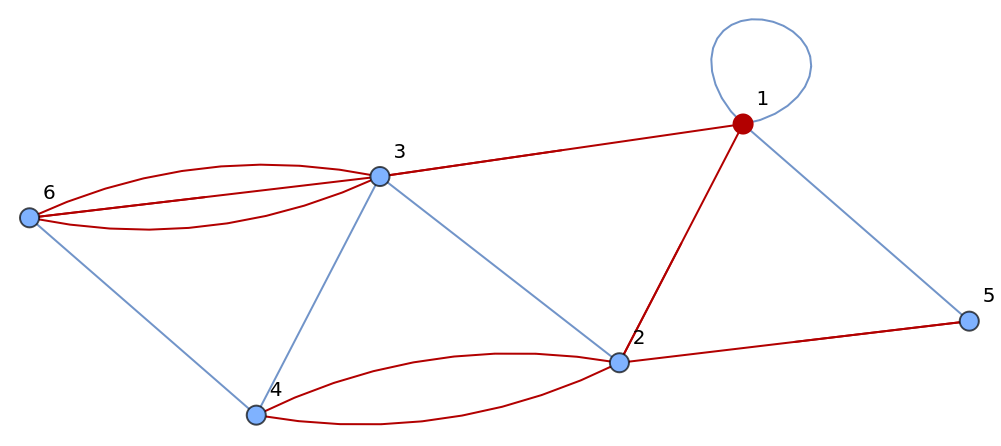
Figure 4. The graph spanning tree (red) returned by BFS function.
As one can see, the tree indeed spans all the vertices of the original graph. The multi edges highlighted are the “artifacts” of HighlightGraph[...] function rather than a flaw of BFS. The latter is easily checked by a stand alone visualization of the tree, Fig. 5.
Figure 5. The stand alone spanning tree of the graph in Fig. 3.
BFS is backbone of the blossom algorithm. To see this, we are going to present a simple “blossom” algorithm for a bipartite graph, which does not contain any odd cycles and requires no flower shrinking. This is the case of so-called the Hungarian algorithm for maximum matching search in a bipartite graph. This very useful from a pedagogical point of view because other tutorials by default imply that the reader is familiar with Hungarian algorithm which is rather strong and optimistic initial assumption.
Like any other function of such kind, our main function realizes the maximum matching search base on Berge’s criterion (Berge1957): the matching is maximum if and only if there are no more augmenting paths in the graph. To understand this criterion, it is, of course, necessary to know what augmenting path is. The augmenting path is a special case of an alternating path that combines matched and unmatched edges sequentially, where the first and the last vertices are uncovered by the matching edges, i.e. they are free vertices. Such special alternating paths can be augmented by swapping matched and unmatched edges, increasing the size of a given matching by one. When no such paths are possible the matching must be a maximum matching. With this sacred knowledge one can write down the following code that reflect this essence:
Thus, all we need now is a function for finding an augmenting path. Based on the definition of an augmenting path, the following function attempts to build alternating paths (or more generally trees) starting from free vertices:
The augmentingpath[...] function terminates and returns an augmenting path whenever it encounter a free vertex as an end point, whereas it growth the tree by two more vertices whenever it encounters a vertex covered by the given matching. In the latter case, the matched vertex is added to the tree together with its mate to which it is linked by the matched edge. If no free vertex is reached from the given one, it takes the next free vertex and try to grow the the alternating tree again. If no augmented path found after trying all free vertices, the function returns an empty path that will terminate the whole search of the maximum matching. In this approach matchings are encoded similar to spanning trees in the parent list. That is, the element position denote the vertex number while the element value is the number of the matching partner vertex.
To see how this works for a bipartite graph, let us take a topologically frustrated hydrocarbon in Fig. 6, which was the first one synthesized (Mishra2020), and find maximum matching for its backbone graph:
Figure 6. A bipartite graph representing carbon skeleton of a topologically frustrated hydrocarbon - Clar’s goblet
Transforming this graph to our maxmatching[...] function input form:
we can run the algorithm:
Now transforming the output back to the graph form:
we obtain the visualization in Fig. 7.
Figure 7. The maximum matching (red) for the Clar’s goblet graph from Fig. 6
By re-running the algorithm we can get a different configuration of matched edges (as per random choice of a starting vertex implemented inside the function) but two vertices will always stay uncovered; see, for example, vertices no. 10 and 28 in Fig. 7.
At this point, it is important to note the following two things. Firstly, for any bipartite graph, one can construct A and D sets from Gallai-Edmonds decomposition by starting growing alternating BFS tree from the vertices not covered by the maximum matching, i.e. again vertices no. 10 and 28 in Fig. 7. In principle, this is doable even manually (Saroka2026) but algorithmic approach is generally more preferable. Secondly, bipartite graphs are the ones that lacks odd cycles. This means that the blossoming procedure is not needed for them. Actually, since topologically frustrated hydrocarbons are bipartite by their definition, all the ingredients presented above are sufficient for topological frustration structural analysis in terms of Gallai-Edmonds decomposition. Yet, a more general algorithm with blossoms is no more complex computationally when applied to bipartite graphs. This means that there is no danger of overloading computer by applying more general algorithm, while the range of treatable problems broadens. Given this, we make some comments on the general implementation of the blossom algorithm without going into details.
Our major comment is regarding realization of odd cycle B shrinking and graph G transformation. In the original paper, Jack Edmonds has the following thoughts regarding this procedure (Edmonds1965, p. 457):
In formal calculation shrinking B in G is an easy operation. Essentially, just assign all the vertices and edges of B a label, b’, and then, until b’ is expanded by erasing these labels, ignore any distinction between vertices labelled b’ and ignore edges joining them to each other.
While semantically this is a well understandable text, the actual action required here is far from being clear. For example, several vertices of the odd cycle can be connected to the same vertex outside the cycle. Shall such edges be preserved or can they all be replaced by a single edge is not clear... Likewise, if several vertices and edges are treated without distinction, won’t this introduce unnecessary extra operations? If the new super vertex replacing a shrunken odd cycle is introduced how the tracking of deleted vertices shall be done? Such simple naive questions can prevent the implementation of the algorithm all together. Given the data presentation adopted, our suggestion would be to shrink blossoms into a new vertex appended to the graph while stripping the blossom vertices from all edges, Fig. 8. The isolated vertices will preserve the vertex numbering in the graph, parent and matching lists, without affecting the final matching found.
Figure 8. The first found blossom, vertices no. 12, 17 and 18, shrinks into an extra vertex no. 19 of the new graph (left) versus the original non-bipartite graph (right). The matching used at this step of the algorithm is highlighted by red color
When the next blossom shrinks, the total graph gains a new vertex, Fig. 9.
Figure 9. The second found blossom, vertices no. 2, 3, and 4, shrinks into an extra vertex no. 20 (left) versus the original graph (right). The matching used at this step is highlighted by red color
This is might be not the most efficient procedure, but it features clarity that often more important than a gentle speed up. In any case, this approach allows to track the changes to extract the final alternating trees from the blossom algorithm, Fig. 10:
Figure 10. The Gallai-Edmonds classification of vertices of the original graph from Figs. 8 and 9 overlaid with the final reduced graph. Orange: D set; violet: A set; yellow: C set. The matching found for the reduced graph is red
The final result, of course, need to be associated with the original graph. We end this technical discussion with the final Gallai-Edmonds decomposition visualized for the original non-bipartite graph, Fig. 11.
Figure 11. The Gallai-Edmonds decomposition of the original graph from Figs. 8 and 9. Orange: D set; violet: A set; yellow: C set
Wolfram Language app
Wolfram Language app
Our app is a graphical user interface (GUI) for building hydrocarbons on a finite piece of the honeycomb lattice of graphene, i.e. nanographenes, and analyzing them on the fly with the above introduced methods and algorithms. Try it below.
Fig. 12. It features two regimes of analysis activated via checkboxes: Gallai-Edmonds decomposition and Sublattice imbalance analysis. Both can be combined for the ease of comparison. Since the property of topological frustration is in the spotlight, only bipartite structures are allowed by design. The results of analysis can be saved into a chosen location as images of five formats: .eps, .pdf, .png, .jpg and .svg. The saved pictures are readily accessible via Open button. Finally, the built nanographenes can be saved as .xyz structures with automatic hydrogen passivation via Export .xyz button. Thus, the app can be used for preparing simple organic structures for quantum mechanical modeling in suits like SIESTA, VASP or Quantum Espresso.
Figure 12. NanographenesBuilder v1.0.0 GUI for bipartite hydrocarbons structure analysis
As an example, let us build the Clar’s goblet from scratch and save it as a graphical output, Fig. 13, and a text file with XYZ coordinates.
Figure 13. Clar’s goblet structural analysis with NanographenesBuilder v1.0.0 (saved result)
The exported structure file “C38_20260614213100.xyz” is
R3Q2: It would be very appreciated (but not obligatory) and impactful to provide for readers some script, program, or computation service for designing embeddings of graphs of required sizes and properties. Such a service could facilitate use of the proposed theory by wide audience and increase number of citations of the paper.
Since the request was not obligatory, a simple promise sufficed to pass the review. However, since the topic is important and, most importantly, interesting, it would be a sin to withdraw from this obligation.
As it usually happens, some unexpected perks popped up along the way in terms of benefits for other lines of research. The Reviewer 2 of another journal paper was curious about precise definition of the topological frustration and suggested some concise variant:
R2Q3: The discussion of the relation between the deficit and the sublattice imbalance remains confusing. To my knowledge: the deficit (defined as the number of sites left unpaired in a maximal matching) is greater than or equal to the sublattice imbalance; topological frustration of second class occurs precisely when this inequality is strict; by the nullity theorem, the deficit guarantees a minimum number of zero-energy states; additional (“supernumerary”) zero modes may appear, but only in non-hexagonal systems. Clarifying these points, and explicitly distinguishing guaranteed from accidental zero modes, would substantially improve the rigor of the discussion.
NanographenesBuilder provides a counter example to the above strict statement, demonstrating that deficit can be larger than the sublattice imbalance in the case when sublattice imbalance is non-zero, Fig. 14:
Figure 14. A graph built on honeycomb lattice that cannot be classified as the topological frustration (class II) due to non-zero sublattice imbalance
Afterword
Afterword
For a long time, topological frustration has been a niche topic for nerdy theorists. The situation has started changing radically in the past few years. A great deal of progress has been achieved in the synthesis of such hydrocarbon molecules:
The 2025 year solely has given us three real species of topologically frustrated nanographenes. These advances fuel growing curiosity in this peculiar area from various research communities. Nowadays, we even have specialized conferences organized exclusively for scientific exchange on this topic:
It must also be noted that considered here topological frustration for finite molecules extended into higher dimensional systems (1D, 2D or 3D) must induce strongly correlated flat band systems (arXiv:2604.01227v3). The last decade has been marked by a search for strongly correlated flat band materials. Superconductivity and exotic quantum states that may arise in such systems urged researchers to undertake significant numerical efforts to reveal potential candidates (Regnault2022) and compile significant databases: Materials Flatband Database. Graph theory plays an increasing role in such efforts (Neves2024). Topological frustration may well play its distinguished role in this vibrant area too.
CITE THIS NOTEBOOK
CITE THIS NOTEBOOK
Graph-theoretic topological frustration in nanographenes: matchings, deficit, and decomposition
by Vasil Saroka
Wolfram Community, STAFF PICKS, June 22, 2026
https://community.wolfram.com/groups/-/m/t/3737934
by Vasil Saroka
Wolfram Community, STAFF PICKS, June 22, 2026
https://community.wolfram.com/groups/-/m/t/3737934