Insights From Chapter 2 of Introduction to Classical and Quantum Computing
by Roman Parker
Intern, Wolfram Research
by Roman Parker
Intern, Wolfram Research
Continuing on from last chapter, we now move into true quantum logic and its fundamentals. We begin with understanding the Bloch Sphere, then move to combining and evaluating quantum states, then finally to quantum circuits and gates. Here, we build up the functions required for quantum computation from Mathematica’s built-ins, although in future sections, the QuantumFramework paclet will likely be used.
Section 2.2: Superposition
Section 2.2: Superposition
Section 2.1 simply serves as an introduction to the topic of the chapter, but 2.2 begins the actual work of explaining Bloch Spheres and quantum superposition.
Intro to The Bloch Sphere
Intro to The Bloch Sphere
Question 2.3
Question 2.3
Here, we were instructed to plot the locations of qubits which were in the states and , a state halfway between them, and two states which were closer to one pole than another. The Bloch Sphere is set up such that is at the “north pole,” is at the “south pole,” and ,, , and are located around the center. For now, the exact numbers of the states don’t matter, put it’s important to know that + is ,- is , + is , and - is .
|0〉
|1〉
|0〉
|1〉
|+〉
|-〉
|〉
|-〉
|0〉
2
|1〉
2
|+〉
|0〉
2
|1〉
2
|-〉
|0〉
2
|1〉
2
|〉
|0〉
2
|1〉
2
|-〉
In[]:=
Graphics3DRGBColor[{1,0,0,.6}],Sphere[],RGBColor[{0,0,1,1}],Sphere[{0,0,1},.1],Text["|0〉",{0,0,1.4}],Green,Sphere[{0,0,-1},.1],Text["|1〉",{0,0,-1.4}],Darker@Yellow,Sphere[{0,1,0},.1],Text"0+1",{0,1.4,0},Darker@Cyan,Sphere[{0,Sqrt[2]/2,Sqrt[2]/2},.1],Text"⬈",{0,Sqrt[2]/2+.2,Sqrt[2]/2+.2},Darker@Magenta,Sphere[{0,Sqrt[2]/2,-Sqrt[2]/2},.1],Text"⬊",{0,Sqrt[2]/2+.2,-Sqrt[2]/2-.2},Lighting"ThreePoint",AxesTrue
1
√2
1
√2
Out[]=

Complex Numbers
Complex Numbers
2.4
2.4
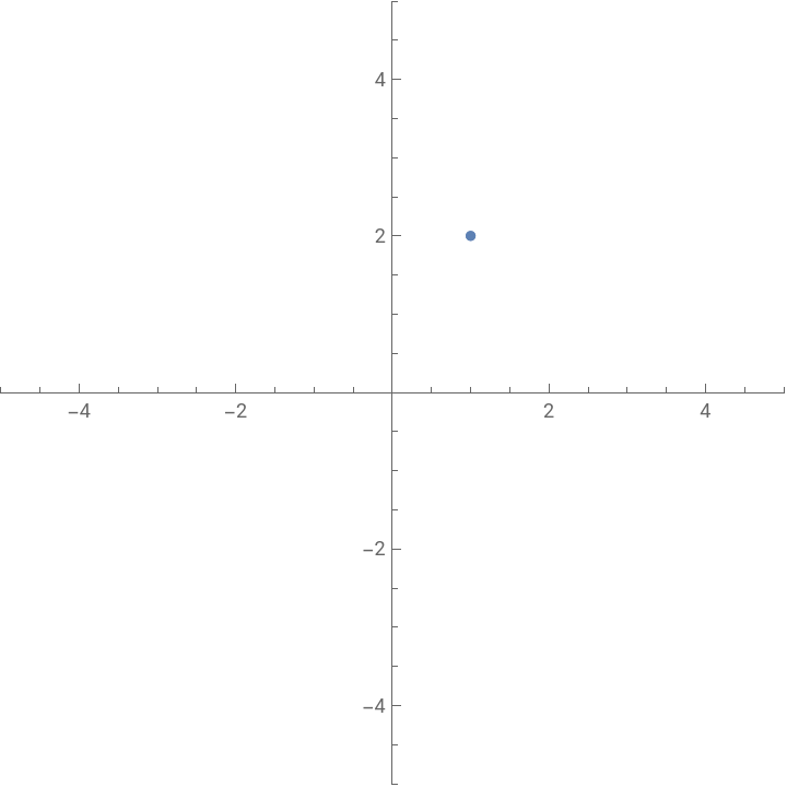
Here, we are supposed to find some important properties of the complex number 1+2. Many of these are quite basic, but they will still be essential in the program to come.
In[]:=
z=1+2I
Out[]=
1+2
In[]:=
Re[z]
Out[]=
1
In[]:=
Im[z]
Out[]=
2
In[]:=
ComplexListPlot[{z},PlotRange{{-5,5},{-5,5}}]
Out[]=
In[]:=
ResourceFunction["ComplexToPolar"][z]
Out[]=
5
ArcTan[2]×
In[]:=
Conjugate[z]
Out[]=
1-2
In[]:=
Norm[z]
Out[]=
5
In[]:=
Norm[z]^2
Out[]=
5
In[]:=
Clear@z;
The norm-square will be especially important, as it it one of the main ways of determining the validity of a quantum state and/or determining the probabilities that come from a measurement.
Section 2.3: Measurement
Section 2.3: Measurement
Basics of Measurement
Basics of Measurement
Exercise 2.6
Exercise 2.6
One of the key takeaways from Section 2.2 is that the probability of measuring a value in a basis is equal to the norm-square of that value’s term. For now, we are simply measuring in and , so that means that the norm-square of the coefficient of a quantum state is the probability of measuring that value.
|0〉
|1〉
In[]:=
z=(1+I*Sqrt[3])/3*|0〉+(2-I)/3*|1〉
Out[]=
1
3
3
)|0〉+2
3
3
In[]:=
Norm[(1+I*Sqrt[3])/3]^2
Out[]=
4
9
In[]:=
Norm[(2-I)/3]^2
Out[]=
5
9
In[]:=
Clear@z
We can see that the probabilities sum to 1, which makes this a valid quantum state (and therefore, a point on the Bloch Sphere). This is the easiest way to test whether a state is valid or not.
Additionally, it is important to remember that if you measure in a basis, it collapses the superposition. This means that all subsequent measurements will still return the same value, even if that value had a low chance of occurring in the first place. For example, say we measured +. There is only a 1 in 81 chance that we obtain , but if we did, all future measurements of this object will still give us that same value.
1
9
|0〉
4+8
9
|1〉
|0〉
Normalization
Normalization
Here, we learn about how to normalize a quantum state so that the probabilities sum to 1.
Exercise 2.8
Exercise 2.8
This problem can relatively easily be solved via Reduce. On more complicated problems, both Solve and Reduce can get hung up and (occasionally) crash your kernel, but Reduce is a little better on that front. Here, we are simply solving for a value of β makes our probabilities function, so there shouldn’t be a problem.
In[]:=
z=(E^(I*Pi/8))/Sqrt[5]*|0〉+β*|1〉
Out[]=
π
8
5
In[]:=
Reduce[{Norm[(E^(I*Pi/8))/Sqrt[5]]^2+Norm[x]^2==1,x>0}]
Out[]=
x
2
5
In[]:=
Clear@z
Exercise 2.9
Exercise 2.9
Here, we are given a more complicated expression and are instructed to find the value which normalizes the equation, along with the probabilities of obtaining and when measured.
|0〉
|1〉
In[]:=
Reduce[{Norm[a*2*E^(I*Pi/6)]^2+Norm[a*-3]^2==1,a>0}]
Out[]=
a
1
13
You may have noticed there’s an a>0 or x>0 in these equations, even though it isn’t called for in most of the cases. This is because there are usually two real solutions (one negative and one positive), and a continuum of complex solutions that we don’t care about, so telling it only to include positive numbers gives us a single solution.
Other Bases
Other Bases
Exercise 2.11
Exercise 2.11
Section 2.4: Bloch Sphere Mapping
Section 2.4: Bloch Sphere Mapping
In this section, we connect together our work on the previous two sections by learning how to take a quantum state and find where it is located on the Bloch Sphere.
Phases
Phases
Exercise 2.13
Exercise 2.13
The easiest way I have found to determine whether states are equivalent or not is to solve for a value that makes the two identical. If this value is a constant, that means that a global phase can simply be added/removed to make the two the same, so they are equivalent. On the other hand, if the result is not constant, there exists a basis which can distinguish the two states.
Spherical Coordinates
Spherical Coordinates
Exercise 2.14
Exercise 2.14
Exercise 2.15
Exercise 2.15
We will skip the last subsection here, as all it talked about was converting from spherical to Cartesian coordinates, which we already did.
Section 2.5: Physical Qubits
Section 2.5: Physical Qubits
This section simply talks about the physics side of things, and details a few objects which can be used as qubits in a quantum computer. It was very short, and had no exercises involving code, so it will be skipped.
Section 2.6: Quantum Gates
Section 2.6: Quantum Gates
This section introduces the main quantum gates, what qualifies as a quantum gate, and how to perform computation using them. Additionally, it shows how to prove that an arbitrary rotation around an axis on the Bloch Sphere is a quantum gate.
Linear Maps
Linear Maps
The definitional property of a quantum gate (compared to a general map) is that they are linear, so that a global phase has no effect, and that the total of the norm-square values is 1, so that the output is a valid quantum state.
Exercise 2.22
Exercise 2.22
Exercise 2.23
Exercise 2.23
Unlike the previous time, there are theoretically a few instances where it behaves as a quantum gate, but it fails for almost all values, so it is once again invalid.
Reversible Gates
Reversible Gates
One of the easiest checks to see if a gate is a valid quantum gate is to see if it is a reversible classical gate. A classical gate is a valid quantum gate IFF it is reversible, and since reversibility is far easier to calculate than amplitude sums, it is quite useful.
Exercise 2.25
Exercise 2.25
Here, we check some gates for reversibility using the techniques from Chapter 1.
One-Bit Gates
One-Bit Gates
Exercise 2.26
Exercise 2.26
Exercise 2.27
Exercise 2.27
This exercise shows us how we can combine together quantum gates which would normally reverse themselves to create something useful.
Exercise 2.28
Exercise 2.28
Here, we take an arbitrary rotation by θ and prove that it is a valid quantum gate. Our first step is to write out what this equation looks like.
Exercise 2.32
Exercise 2.32
Here, we are working with the Hadamard gate, which is a rotation on a combined X+Z axis. Our goal is simple: Show that for arbitrary terms, HXH is the same as Z.
This is our first identity that we have defined,which will be useful later on for creating circuits.
Generalizing Gates
Generalizing Gates
Here, we look at creating arbitrary rotations on all three axes and how to define them as quantum gates.
Exercise 2.34
Exercise 2.34
Here, we create a more arbitrary rotation around the axis. We start by determining the direction vector and confirming that it, in fact, does meet the requirement of being a unit vector. Since we are rotating about the Z axis, X and Y can be 0 while Z is 1.
Next, we define a function which can convert an arbitrary rotation θ around any axis into a quantum gate. θ represents our rotation angle, ⋁ represents our input terms to the gate, x, y, and z represent the values of the direction vector on each of those axes, and γ represents a global phase, which can be set to any value but allows us to simplify and compare gates in a significantly easier way.
This is a bit complicated-looking, but when we convert it into exponential form, things do simplify a bit.
By doing this, we have shown that our new rotation gate is identical to the T Gate other than a global phase.
Section 2.7: Quantum Circuits
Section 2.7: Quantum Circuits
In this section, we create a very basic quantum circuit by chaining gates and find what probabilities each output has.
Creating Circuits
Creating Circuits
Exercise 2.36
Exercise 2.36
This concludes Chapter 2 of Introduction to Classical and Quantum Computing.