We compute the rate of absorption and the concentration profile of a solute of limited solubility, which diffuses into a semi-infinite domain and undergoes a first-order reaction.
We compute and plot the concentration profile for two different cases:
1- The first case is when penetration depth is limited by diffusion.
2- In the second case, penetration depth is limited by reaction.
1- The first case is when penetration depth is limited by diffusion.
2- In the second case, penetration depth is limited by reaction.
We also compare our results with the analytical solution derived in Ref. 1. We find that both results are in agreement.
Governing equation and boundary conditions are:
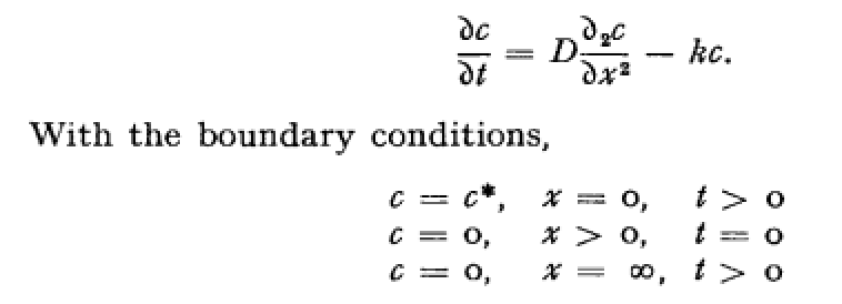
Analytical solution was derived by P. V. Danckwerts in Ref.1.
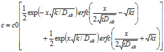
Diffusion coefficient is . Rate constant is k. c0 is surface concentration.
D
AB
In[]:=
D
AB
In[]:=
k=35;
In[]:=
c0=3 10^-2;
Case 1: Penetration depth is limited by reaction: >>1
δ
d
δ
r
In[]:=
t=10^2;
In[]:=
δ
d
D
AB
Out[]=
0.000387298
In[]:=
δ
r
D
AB
Out[]=
6.54654×
-6
10
In[]:=
δ
d
δ
r
Out[]=
59.1608
In[]:=
c=.;t=.;
Solving the governing equation with NDSolve using the following boundary condition c[10 ]=0 with ~.
δ
r
δ
r
-5
10
In[]:=
sol=NDSolve[{D[c[t,x],{t,1}]D[c[t,x],{x,2}]-kc[t,x],c[0,x]c0Exp[-10^20x],c[t,0]c0,c[t,110^-4]0},c[t,x],{x,0,110^-4},{t,0,100}]
D
AB
Out[]=
c[t,x]InterpolatingFunction[t,x]


In[]:=
plt1=Plot[Chop[c[t,x]/.sol/.t->10^2],{x,0,1 10^-4},PlotRange->{0,0.03},PlotStyle->{Thick,RGBColor[1,0,0]},Frame->True,
FrameLabel->{Style["position",16],Style[" concentration ",16]},GridLines->Automatic,AspectRatio->1]
FrameLabel->{Style["position",16],Style[" concentration ",16]},GridLines->Automatic,AspectRatio->1]
Out[]=
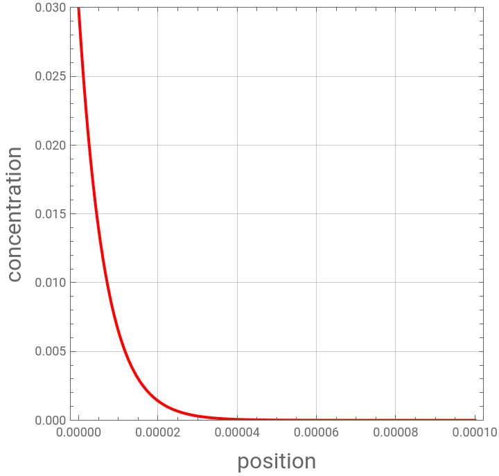
We plot Danckwerts' analytical solution
In[]:=
c=c0(0.5Exp[-x(k/)^0.5]Erfc[x/(2(t)^0.5)-(tk)^0.5]+0.5Exp[x(k/)^0.5]Erfc[x/(2(t)^0.5)+(tk)^0.5])
D
AB
D
AB
D
AB
D
AB
Out[]=
3
100
-152753.x
0.5
t
12909.9x
0.5
t
152753.x
0.5
t
12909.9x
0.5
t
In[]:=
plt2=Plot[Chop[c/.t->10^2],{x,0,10^-4},PlotRange->{0,0.03},PlotStyle->{Dashed,RGBColor[0,0,1]},Frame->True,
FrameLabel->{Style["position",16],Style[" concentration ",16]},GridLines->Automatic,AspectRatio->1]
FrameLabel->{Style["position",16],Style[" concentration ",16]},GridLines->Automatic,AspectRatio->1]
Out[]=
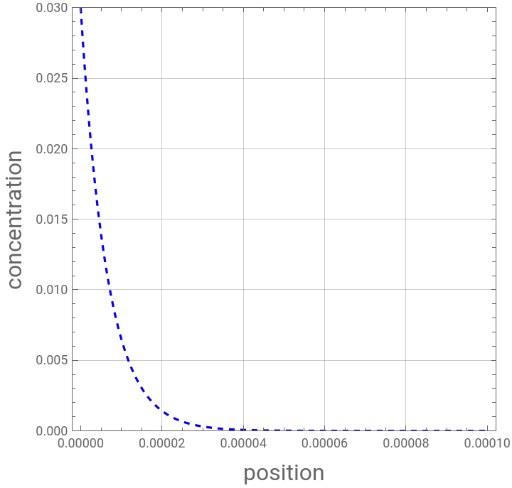
Both methods give the same concentration profile
In[]:=
Show[plt1,plt2]
Out[]=
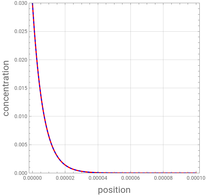
Let us determine the quantity of solute absorbed, Q. Using the analytical concentration expression, one gets (see Ref.1) :1/ the Rate of absorption :2/ the quantity of solute absorbed, Q.


In[]:=
D
AB
In[]:=
k=.;
In[]:=
c0=.;
In[]:=
t=.;
In[]:=
c=c0(1/2Exp[-xSqrt[k/]]Erfc[x/(2Sqrt[t])-Sqrt[tk]]+1/2Exp[xSqrt[k/]]Erfc[x/(2Sqrt[t])+Sqrt[tk]])
D
AB
D
AB
D
AB
D
AB
Out[]=
c0Erfc-+Erfc
1
2
-x
k
D
AB
kt
+x
2
t
D
AB
1
2
x
k
D
AB
kt
+x
2
t
D
AB
In[]:=
rateofabsorption=-D[c,{x,1}]/.x0//FullSimplify
D
AB
Out[]=
c0kErf[
kt
]k
D
AB
c0
-kt
t
D
AB
π
tIn[]:=
D
AB
In[]:=
k=35;
In[]:=
c0=3 10^-2;
In[]:=
t=.;
In[]:=
Qanalytical=NIntegrate[rateofabsorption,{t,0,10^2}]
Out[]=
0.000687386
In[]:=
Qanalytical=Quiet[c0Sqrt[/k]((kt+1/2)Erf[kt]+Sqrt[kt/Pi]Exp[-kt])/.t10^2.]
D
AB
Out[]=
0.000687485
Case 2: Penetration depth is limited by diffusion: <<1
δ
d
δ
r
In[]:=
t=10^-7;
In[]:=
c=.;t=.;
In[]:=
plt1=Plot[Chop[c[t,x]/.sol/.t->10^-7],{x,0,1 10^-7},PlotRange->{0,0.03},PlotStyle->{RGBColor[1,0,0],Thick},
FrameLabel->{Style["position",16],Style[" concentration ",16]},Frame->True,GridLines->Automatic,AspectRatio->1]
FrameLabel->{Style["position",16],Style[" concentration ",16]},Frame->True,GridLines->Automatic,AspectRatio->1]
Let us plot Danckwerts' analytical solution:
In[]:=
plt2=Plot[Chop[c/.t->10^-7],{x,0,1 10^-7},PlotRange->{0,0.03},PlotStyle->{Dashed,RGBColor[0,0,1]},
FrameLabel->{Style["position",16],Style[" concentration ",16]},Frame->True,GridLines->Automatic,AspectRatio->1]
FrameLabel->{Style["position",16],Style[" concentration ",16]},Frame->True,GridLines->Automatic,AspectRatio->1]
Both methods give the same concentration profile
In[]:=
Show[plt1,plt2]
References
References
◼
[1] P. V. Danckwerts, Absorption by simultaneous diffusion and chemical reaction, Trans. Faraday Soc., 46, pp. 300-304 (1950).
◼
[2] C. J. Geankoplis, Transport Processes and Unit Operations, 3rd edition, Prentice Hall, 1993.
CITE THIS NOTEBOOK
CITE THIS NOTEBOOK
Unsteady-State Diffusion and Reaction in a Semi-infinite Medium
by Housam Binous and Ahmed Bellagi
Wolfram Community, STAFF PICKS, February 18, 2024
https://community.wolfram.com/groups/-/m/t/3125417
by Housam Binous and Ahmed Bellagi
Wolfram Community, STAFF PICKS, February 18, 2024
https://community.wolfram.com/groups/-/m/t/3125417