Molecular dynamics simulations (MD) and Monte Carlo simulations (MC) are the two dominant ways to simulate molecular systems in chemical thermodynamics. This software package contains the executable algorithm for a Monte Carlo simulation in the Gibbs ensemble (GEMC). The software can be used to simulate pure components and binary mixtures of rigid partially charged molecules in the NVT and NPT ensemble. The OPLS force field is used for calculating intermolecular interactions, and different combining rules can be used for unlike pair interaction parameters. Both the Ewald and the Wolf summation can be used for calculation of the electrostatic long-range correction. Simulations can be conducted using conventional as well as more advanced methods for insertions like the identity swap method for binary mixtures and the continuous fractional component (CFC) method. It is possible to auto-calibrate simulation parameters such as trial move limits, number of attempted transfers and species selection pseudo-probability for transfers to ensure sufficient successful trial moves. A simulation is conducted in three phases: (i) the warm-up, (ii) the equilibration, and (iii) the production phase. A schematic of the GEMC method is displayed in the figure above. CITATION: Michael Haring, Niklas Mayr, Sebastian Thaler, Thomas Steiner, Thomas Wallek, “Gibbs Ensemble Monte Carlo Simulations for Fluid Phase Equilibria” from the Notebook Archive (2022), https://notebookarchive.org/2022-11-6ger7tx
All needed packages and files: https://notebookarchive.org/2022-11-6ger7tx/2022-11-6ger7tx_Supplements.zip
All needed packages and files: https://notebookarchive.org/2022-11-6ger7tx/2022-11-6ger7tx_Supplements.zip
After unpacking the zip archive see Documentation - v3.1.0.pdf for complete information about Gibbs Ensemble Monte Carlo Simulations for Fluid Phase Equilibria and instructions for the included Wolfram Language code.
This notebook is - in contrast to the others - intentionally based on the *.nb format. Thereby the results are saved if the notebook is closed and can be re-examined any-time, for example when simulation results are investigated for plausibility. It is recommended to execute entire sections or subsections, to ensure all necessary code is executed.
In[]:=
SetDirectory[NotebookDirectory[]];Get[FileNameJoin[{"pkg","PropertyPackage.wl"}]]Get[FileNameJoin[{"pkg","ForceFieldOPLS.wl"}]]Get[FileNameJoin[{"pkg","ChemicalThermoPackage.wl"}]]
Pure Component
Component Name and Label
Component Name and Label
Enter the name of the component and the OPLS-label.
The check will tell if they are present in the packages and additional information can be extracted.
Critical point data and Antoine parameter will be extracted from the ‘physicalPropertyData’.
The LJ parameters will be extracted from ‘oplsNonBonded’.
The check will tell if they are present in the packages and additional information can be extracted.
Critical point data and Antoine parameter will be extracted from the ‘physicalPropertyData’.
The LJ parameters will be extracted from ‘oplsNonBonded’.
◼
Check-Function
In[]:=
component="Argon";(*nameofthecomponentintheProperty-Package*)labelLj="Ar,Tan";(*nameoftheOPLS-labelintheForceFieldOPLS-Package*)CheckPureInput[]
Component was found in 'physicalPropertyData'
Label was found in 'oplsNonBonded'
Experimental and Physical Property Data
Experimental and Physical Property Data
In this section, experimental data can be entered and compared to the Antoine equation and Thol2016 EoS.
It will also be available in further sections. Be sure to update this section for your investigated component.
It will also be available in further sections. Be sure to update this section for your investigated component.
Experimental Data
Experimental Data
literature references:Argon ... CRC Handbook,99th Ed.,2019-2019Ethane ... Horstmann S., et.al., GPA Research Rep., Rep.No. RR-203, 1-127, 2010 CRC Handbook, 99th Ed., 6-125 - 6-127
saturation densities: rhoSatExp = {T[K], [mol/dm³], [mol/dm³]}saturation pressure: pSatExp = {T[K], P[bar]}
Vap
ρ
Liq
ρ
In[]:=
rhoSatExp=<|"Argon"->{{83.81,0.102,35.471},{90.,0.186,34.52},{100.,0.422,32.893},{110.,0.833,31.1150},{120.,1.505,29.113},{130.,2.593,26.735},{140.,4.478,23.623},{150.,9.875,17.032},{150.69,13.407,13.407}},"Ethane"->{{245.00,0.715,15.0283},{262.53,1.19721,14.0805},{278.61,1.95544,12.8168}}|>;pSatExp = <|"Argon"->{{83.806,0.68891},{88.806,1.1842},{93.806,1.9146},{98.806,2.9414},{103.81,4.33},{108.81,6.1474},{113.81,8.4634},{118.81,11.349},{123.81,14.877},{128.81,19.125},{133.81,24.174},{138.81,30.118},{143.81,37.071},{148.81,45.197}},"Ethane"->{{120.,0.004},{140.,0.038},{160.,0.215},{180.,0.787},{200.,2.17},{220.,4.92},{240.,9.67},{260.,17.12},{280.,28.06},{300.,43.55}}|>;
Extract LJ Parameters
Extract LJ Parameters
In[]:=
(*obtain LJ parameters*){σ(*[Å]*),ϵ(*[kcal mol^-1]*)} = oplsNonBonded[labelLj][[{2,3}]];(*conversion factors for T from K > reduced Lj Units*)tLjRedFac = 1 (*K*)/(ϵ (*kcal /mol*) *4184 (*J /mol*) /nAvogadro (*J /1*) /kB (*1*)) (**) ;(*conversion factors for rho(T)*)rhoLjRedFac = 1 (*mol/*) *nAvogadro (*1/*) *10^(-27) (*1/)*) *σ^3 (*1*);(*conversion factors for rho(T) and p(T) data*)pLjRedFac = 1 (*bar*) * (*Pa*) *(σ (*A*) * (*m*))^3 (**) (ϵ (*kcal /mol*) *4184 (*J /mol*) /nAvogadro (*J /1*));
*
t
3
dm
3
dm
3
A
5
10
-10
10
3
m
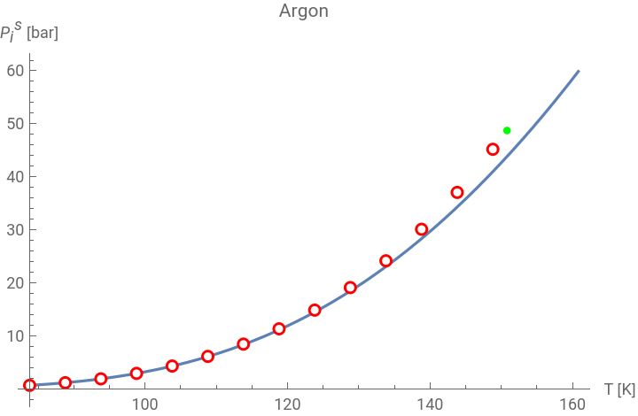
Compare Experimental Data with Antoine
Compare Experimental Data with Antoine
In[]:=
IfKeyExistsQ[physicalPropertyData,component] && KeyExistsQ[physicalPropertyData[component],"antoineParameters"] && KeyExistsQ[pSatExp,component], Show PlotpAntoine[x,physicalPropertyData[component,"antoineParameters",1, #]&/@{"A","B","C"},"log10"] ,{x,Min[pSatExp〚component,All,1〛],physicalPropertyData[component,"tCrit"]+10} ,PlotLegends{"Antoine"},PlotLabelcomponent,AxesLabel{"T [K]"," [bar]"} , ListPlot[pSatExp[[component]],PlotMarkers"OpenMarkers",PlotLegends{"Experimental"},PlotStyle{Red}], ListPlot[{{physicalPropertyData[component,"tCrit"],physicalPropertyData[component,"pCrit"]}},PlotLegends{"Critical point"},PlotStyle{Green}] , Print@Style["No Antoine parameter or experimental data are available!",Bold,14]
s
P
i
Out[]=


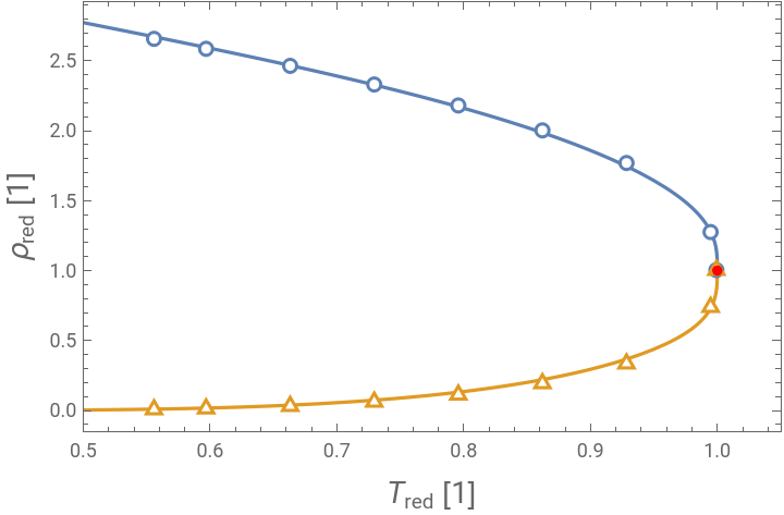
Does the component behave like a Lennard-Jones fluid?
Does the component behave like a Lennard-Jones fluid?
The experimental data is compared to the prediction of the Thol2016 EoS for LJ-fluids in reduced units. =T/ =ρ/The experimental data is reduced using the critical point from the “physicalPropertyData”.
T
red
T
C
ρ
red
ρ
C
In[]:=
IfKeyExistsQ[physicalPropertyData,component] && AllTrue[(KeyExistsQ[physicalPropertyData[component],#]&/@{"vCrit","tCrit"}),TrueQ], Module{tCrit,vCrit}, tCrit = physicalPropertyData[component,"tCrit"]; vCrit = physicalPropertyData[component,"vCrit"]; Show Plot{ρSatLiqRedLJ[tRed],ρSatVapRedLJ[tRed]},{tRed,0.5,1.} (*,PlotLabel "Reduced Density at Saturation"*) ,FrameTrue,FrameLabel(Style[#, 14]&/@{ " [1]", " [1]"}) ,PlotLegends{"Saturated Liquid, Thol 2016 LJ-Fluid EOS","Saturated Vapor, Thol 2016 LJ-Fluid EOS"} ,PlotRange{{0.5, 1.05}, Automatic} , ListPlot Transpose[{rhoSatExp〚component,All,1〛/tCrit,rhoSatExp〚component,All,3〛*vCrit}], Transpose[{rhoSatExp〚component,All,1〛/tCrit,rhoSatExp〚component,All,2〛*vCrit}] ,PlotLegends{"Saturated Liquid, Experimental","Saturated Vapor, Experimental"} ,PlotMarkers"OpenMarkers" , ListPlot[{1.,1.},PlotStyle{Red,PointSize[0.015]},PlotLegends{"Critical point"}] , Print@Style["No critical point data available!",Bold,14]
T
red
ρ
red
Out[]=


Simulation point proposal, based on Thol2016 EoS
Simulation point proposal, based on Thol2016 EoS
The EoS by Thol uses LJ-reduced units for temperature, pressure and density which are denoted with an uppercase Asterisk. = = =ρ*
*
T
T*
k
B
ε
*
P
P*
3
σ
ε
*
ρ
3
σ
State Definition
State Definition
Choose the temperature between the boiling temperature and the critical temperature of the LJ-fluid
In[]:=
Grid[{{"",0.5*tCritLJ/tLjRedFac,"K"},{"",1.0*tCritLJ/tLjRedFac,"K"}},FrameAll,Spacings->{1, Automatic}]
T
boil
T
C
Out[]=
T boil | 77.0814 | K |
T C | 154.163 | K |
Calculation and Visualization
Calculation and Visualization
The following simulation setup is calculated under the assumption that the result of the Thol2016 EoS is the final value of the densities.
We assume a final distribution of the molecules where 40% of the total molecules is in the vapor phase and 60% of the total molecules are in the liquid phase.
We calculate the theoretical total volume of this simulation setup and use it for a setup with equal amounts of molecules in each box as well as the same initial density.
-------------------------------------------------------------------------------
-------------------------------------------------------------------------------
Simulation point proposal, based on SRK EoS
Simulation point proposal, based on SRK EoS
State Definition
State Definition
Choose the temperature between the boiling temperature and the critical temperature
Calculation and Visualization
Calculation and Visualization
Binary Mixture with Critical Point Data
Component Names
Component Names
Experimental and Physical Property Data
Experimental and Physical Property Data
Mind to update the experimental data according to the set components!
Saturation Pressure
Saturation Pressure
Experimental Data
Experimental Data
Compare Antoine with Experimental Data
Compare Antoine with Experimental Data
Mixture Data
Mixture Data
The {Pxy}-diagram for experimental temperature using Raoult-Dalton
The {Pxy}-diagram for experimental temperature using Raoult-Dalton
Estimation using Raoult-Dalton for molar fraction
Estimation using Raoult-Dalton for molar fraction
State Definition
State Definition
Calculation and Visualization
Calculation and Visualization
Binary Mixture of LJ-fluids
The aim of this section is to give aid to choose the initial Temperature and Pressure for the simulation as well as appropriate starting values for the molar density and molar fraction of the boxes.
The LJ-reduced values marked with an asterisk are calculated using the LJ-Parameters as follows:
The LJ-reduced values marked with an asterisk are calculated using the LJ-Parameters as follows:
The index 11 refers to the interaction parameters between two particles of the first species in the system.
The density is reduced using a mixture parameter that can be calculated as follows:
The density is reduced using a mixture parameter that can be calculated as follows:
Experimental Data (Saturation Pressure)
Experimental Data (Saturation Pressure)
Visualisation
Visualisation
Credits
◼
Version 2.0: Niklas Mayr
◼
Version 3.1: Michael Haring
CITE THIS NOTEBOOK
CITE THIS NOTEBOOK
Gibbs Ensemble Monte Carlo simulations for fluid phase equilibria: experimental data and estimations
by Michael Haring, Niklas Mayr, Sebastian Thaler, Thomas Steiner, Thomas Wallek
Wolfram Community, STAFF PICKS, March 13, 2026
https://community.wolfram.com/groups/-/m/t/3660101
by Michael Haring, Niklas Mayr, Sebastian Thaler, Thomas Steiner, Thomas Wallek
Wolfram Community, STAFF PICKS, March 13, 2026
https://community.wolfram.com/groups/-/m/t/3660101