Get Data (2015-2020) From TxDOT CRIS
Get Data (2015-2020) From TxDOT CRIS
All data downloaded from TxDOT. The data file is attached below. Please make sure to put it in the same directory with this notebook for the next code line to work.
Data (as csv) imported:
Data (as csv) imported:
SetDirectory[NotebookDirectory[]]
D12Crashes=Import["D12CrashesFull.csv"];
In[]:=
D12Crashes[[24;;-1]]//Length
Out[]=
34084
34084 crashes (although each one is counted [at least] twice, one for each vehicle involved)
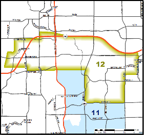
Map of Dallas’ District 12 Boundary
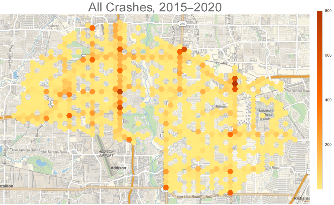
Heatmap: All Crashes 2015-2020
Heatmap: All Crashes 2015-2020
Let’s take the crash data, extract the latitude and longitude, and make a GeoHistogram in order to visualize the most frequent areas of crashes:
In[]:=
GeoHistogram[Map[#[[13;;14]]&,D12Crashes[[24;;-1]]],Quantity[1000,"Feet"],PlotLegendsAutomatic,GeoBackground"StreetMap",PlotStyleOpacity[1.0],ImageSize800,PlotLabelStyle["All Crashes, 2015-2020",FontSize32]]
Out[]=
Finding Top Intersections
Finding Top Intersections
Let’s put all the crashes into hexagonal bins of radius 1000ft (using a neat function from the function repository):
(note: 1/364.5672 decimal degree = 1000 feet)
(note: 1/364.5672 decimal degree = 1000 feet)
In[]:=
D12CrashesHexBins=ResourceFunction["HextileBins"][Map[#[[13;;14]]&,D12Crashes[[24;;-1]]],1/364.5672];
This results in 737 bins:
In[]:=
D12CrashesHexBins//Length
Out[]=
737
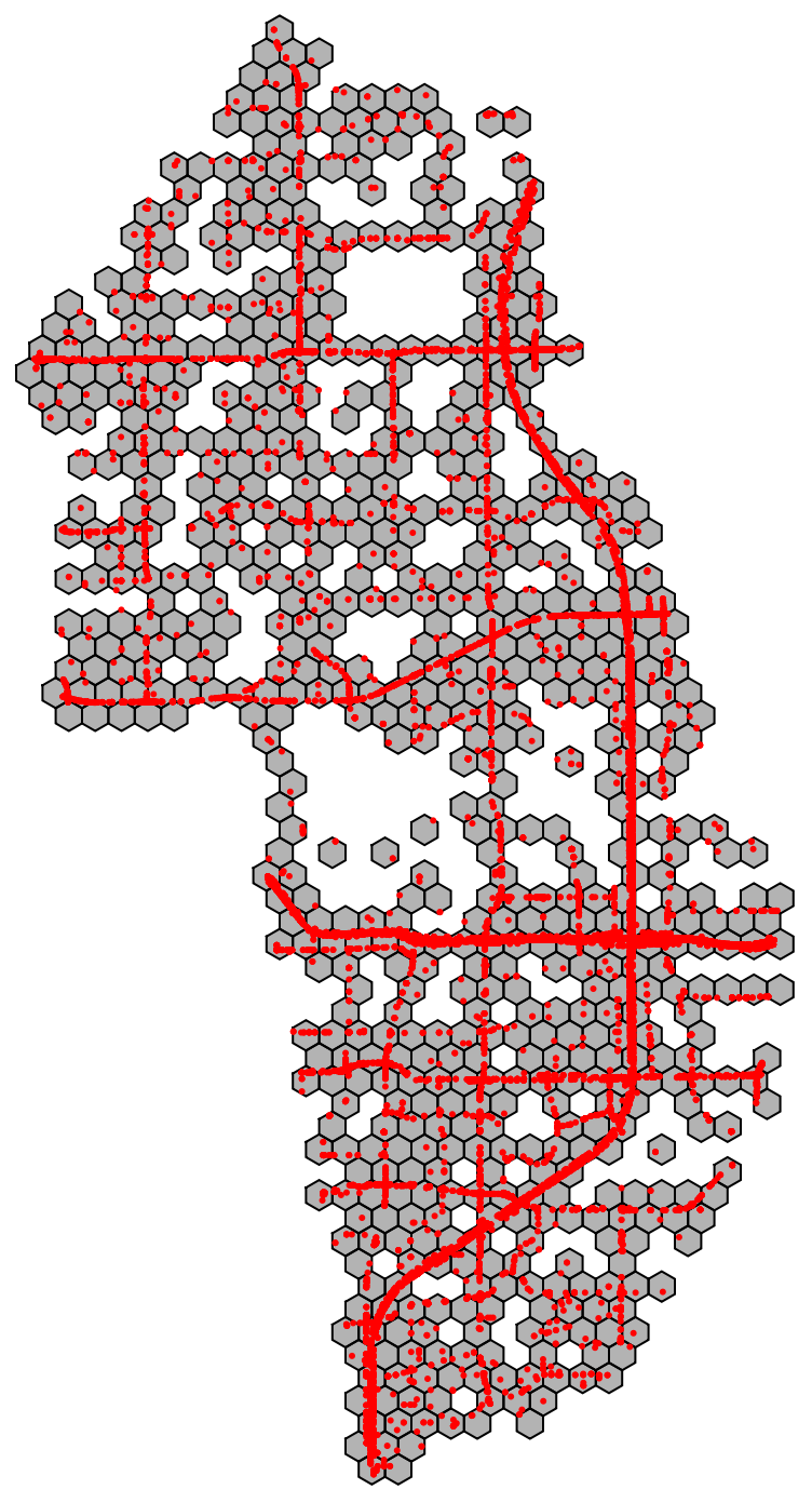
Let’s visualize it (notice how it’s rotated):
In[]:=
Graphics[{EdgeForm[Black],FaceForm[Opacity[0.3]],Keys@D12CrashesHexBins,Red,Point[Map[#[[13;;14]]&,D12Crashes[[24;;-1]]]]}]
Out[]=
Let’s look at the distribution of crashes:
In[]:=
(((Table[D12CrashesHexBins[[x]],{x,1,737}]//Sort//Reverse)/34084.0)[[1;;20]])//Total//PercentForm
Out[]//PercentForm=
30.57%
So the top 20 intersections account for 30% of all accidents.
Let’s see the top 20:
Let’s see the top 20:
In[]:=
Take[D12CrashesHexBins,{4}]
Out[]=
Polygon425


In[]:=
Map[First,%120]
Out[]=
Polygon936,Polygon793,Polygon712,Polygon673,Polygon669,Polygon601,Polygon547,Polygon523,Polygon492,Polygon464


In[]:=
(SortBy[Table[{Take[D12CrashesHexBins,{x}],D12CrashesHexBins[[x]]},{x,1,737}],Last]//Reverse)[[1;;10]]
Out[]=
Polygon936,936,Polygon793,793,Polygon712,712,Polygon673,673,Polygon669,669,Polygon601,601,Polygon547,547,Polygon523,523,Polygon492,492,Polygon464,464
Let’s now make a geo-visualization of where these intersections are, with their labeled rankings:
Areas where you are most likely to have a crash: