ABSTRACT (original article): We consider the dynamics of a bead that slides frictionlessly along a rotating slanted wire of infinite length and finite moment of inertia under the influence of uniform gravity. Since the wire is frictionless and external forces are absent, energy and angular momentum are conserved, and the angular velocity of the wire may increase or decrease as the bead and the wire exchange energy. Assuming that the bead is initially at rest along the wire, this paper characterizes all possible trajectories of the bead along the wire, which may be constant, divergent, oscillatory, or convergent. CITATION (original article): Kouba, O., Bernstein, D.S. On the Dynamics of a Bead Sliding on a Freely Rotating Slanted Wire. J Nonlinear Sci 34, 57 (2024). https://doi.org/10.1007/s00332-024-10036-4
The movement of the bead on a freely rotating slanted wire making angle with the horizontal plane is studied.
The equations of the movement are transformed to a standard form. It is reduced to the study of the differential equation
ϕ
The equations of the movement are transformed to a standard form. It is reduced to the study of the differential equation
′′
z
z
2
(1+)
2
z
z
0
′
z
where and . is the initial angular speed of the bead. is the initial position of the bead on the wire. is a constant that depends on the system.The standard angle of rotation of the wire is then given by .The different cases correspond to those considered in the paper.
a
z
e
2
1+
2
z
0
z
e
1
2
ηω
0
ω
0
z
0
η
Θ(t)du
ω
0
t
∫
0
1+
2
z
0
1+(u)
2
z
Initialization
g[z0_]:=;Q[z_,z0_,a_]:=+1-;η=1;ϕ=π/3;(*Thewireisslantedwithananglewiththehorizontalplane*)
1+
2
z0
4
1+
-z02
z0
2
z
z+z0
2a(1+)
2
z0
ϕ
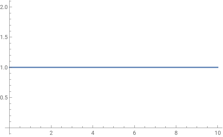
Case 1 corresponds to the stationary orbit of the bead.
When=, simulation confirms that the solution is .
When
z
0
z
e
z:t↦
z
0
(*Case1:z0=ze=,Equilibrium*)z0=1;ze=1;a=;s1=NDSolvez''[t]-==-a,z[0]==z0,z'[0]==0,z,{t,0,10};Plot[{Evaluate[z[x]/.s1]},{x,0,10},PlotRangeAll]
1
η
2
ω0
ze
2
(1+)
2
z0
z[t]
2
(1+)
2
z[t]
Out[]=
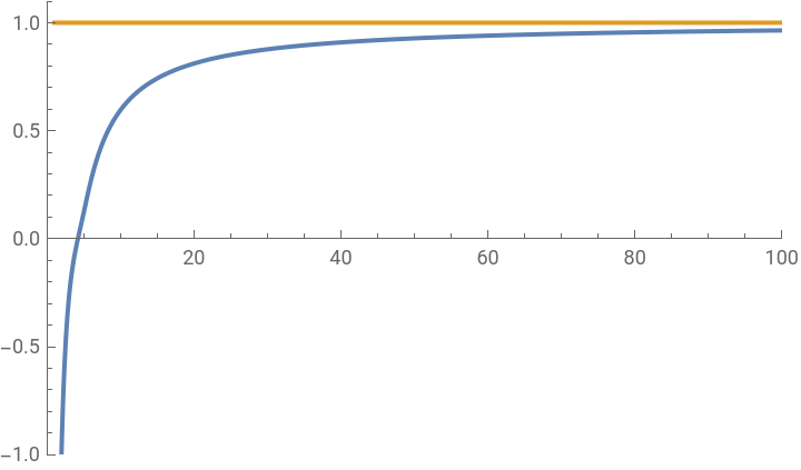
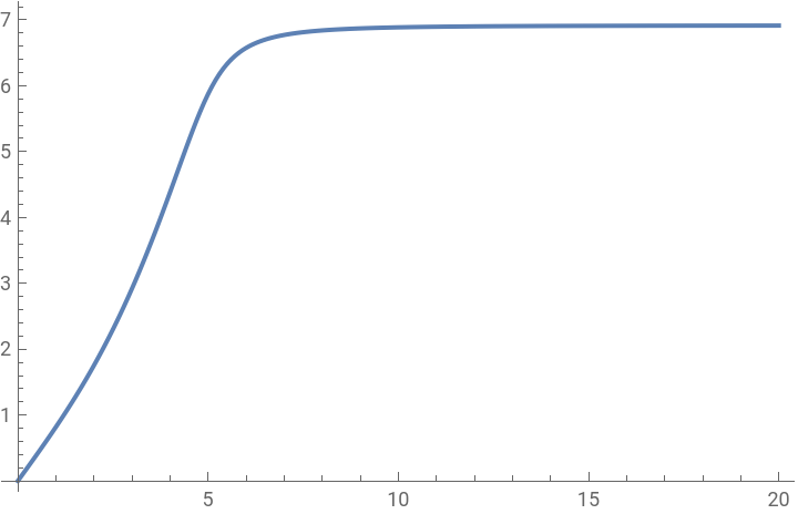
Case 2.1 corresponds to .In this example and ≈1.56; ■ The first plot confirms that the solution for large . ■ The second plot shows how Θ rapidly approaches a final ≈6.91. ■ The third plot shows the position of the bead on the cone drawn by the rotating wire.
g()<
z
0
z
e
g()≈1.2
z
0
z
e
z(t)∼-
a
2
2
t
t
Θ
∞
Case 2.1 :
g()<
z
0
z
e
z0=1;ω0=;ze=;Print["z0 = ",z0]Print["ze = ",ze]Print["g[z0]<ze is ",g[z0]<ze]a=;s21=NDSolvez''[t]-==-a,z[0]==z0,z'[0]==0,z,{t,0,1000};(*Firstplot*)Plot,1,{x,1,100},PlotRange->{{0,100},{-1,1.1}}(*secondplot*)Theta[t_]:=NIntegrateEvaluateω0/.s21,{x,0,t}[[1]];L=Table[{t,Theta[t]},{t,0,20,0.1}];ListPlot[L,Joined->True](*Thirdplot*)tmax=6;L3d=Table[{Point[Flatten[{Cos[Theta[t]]Cos[ϕ],Sin[Theta[t]]Cos[ϕ],Sin[ϕ]}Evaluate[z[t]/.s21][[1]]]]},{t,0,tmax,0.1}];c1={EdgeForm[],Opacity[0.5],LightRed,Cone[{{0,0,Sin[ϕ]}(1.2)Evaluate[z[0]/.s21][[1]],{0,0,0}},Cos[ϕ](1.2)Evaluate[z[0]/.s21][[1]]]};c2={EdgeForm[],Opacity[0.5],LightRed,Cone[{{0,0,Sin[ϕ]}(1.2)Evaluate[z[tmax]/.s21][[1]],{0,0,0}},Cos[ϕ](1.2)Abs[Evaluate[z[tmax]/.s21][[1]]]]};Show[Graphics3D[{L3d,c1,c2}],Boxed->False]
8
10
1
η
2
ω0
ze
2
(1+)
2
z0
z[t]
2
(1+)
2
z[t]
Evaluate[z[x]/.s21]
-(a/2)
2
x
(1+)
2
z0
1+
2
z[x]
z0 = 1
ze =
25
16
g[z0]<ze is True
Out[]=
Out[]=
Out[]=

◼
The second plot shows the trade between the Energy of the bead (blue) and the energy of the wire (orange), while the total energy of the system is constant (green).
◼
The third plot shows the position of the bead on the cone drawn by the rotating wire.
◼
The second plot shows the position of the bead on the cone drawn by the rotating wire.
◼
The third plot shows the position of the bead on the cone drawn by the rotating wire.
CITE THIS NOTEBOOK
CITE THIS NOTEBOOK
On the dynamics of a bead sliding on a freely rotating slanted wire
by Omran Kouba and Dennis S. Bernstein
Wolfram Community, STAFF PICKS, May 6, 2024
https://community.wolfram.com/groups/-/m/t/3171119
by Omran Kouba and Dennis S. Bernstein
Wolfram Community, STAFF PICKS, May 6, 2024
https://community.wolfram.com/groups/-/m/t/3171119