Topological Kleene Field Theories (TKFTs) represent a new framework in the world of computational theory, where computations are introduced as flows in cobordisms. In this work, we fully realize this construction into concrete terms, explicitly computing the smooth dynamics that simulates any Turing machine, and hence illustrating how TKFTs are Turing complete.
Introduction
Introduction
Topological Kleene Field Theories (TKFTs) constitute a recently developed framework [2] that reimagines the notion of computation through the language of smooth bordisms and continuous flows. By establishing a bridge between geometry and computation, TKFTs provide a means to interpret computable functions as dynamical evolutions and topological decompositions. As highlighted by the authors, this perspective carries significant consequences for dynamical systems theory. In particular, it reveals that certain dynamical questions, such as whether a trajectory reaches a given point or becomes trapped, are inherently undecidable, reflecting the undecidability of the halting problem. Moreover, the authors demonstrate that the class of smooth vector fields is Turing complete: any computable function can be realized as the flow of a vector field on an appropriate bordism.
In this paper, the proof of this Turing completeness relies on representing a Turing machine by its underlying graph, which is then “thickened” to a smooth manifold. By encoding the tape as a point within a disk via a Cantor set–type embedding, they show that the fundamental operations of the machine can be implemented through suitable diffeomorphisms. However, explicit formulas for these diffeomorphisms, as well as the detailed construction of the corresponding cobordisms, are not provided in the original work.
In a previous project [3], we explicitly computed these flows, and hence simulated the computational dynamics on the cobordisms corresponding to certain simple Turing machines. This project constitutes a direct continuation of the previous work, as our objective here has been to generalize the previous construction and expand it so any Turing machine can be simulated, and hence explicitly demonstrate that TKFTs are indeed Turing complete, as proved in [2].
The structure of this project will consist first on a brief introduction to Topological Kleene Field Theories (TKFTs), although we refer to the reader to the previous paper, [3] for a detailed explanation. Then, we will present the detail construction for the simulation of any Turing machine. Finally, we will show some particular examples of simulations for Turing machines with different number of states.
How Topological Kleene Field Theories work
How Topological Kleene Field Theories work
In this section, we will briefly explore how TKFTs work. As previously mentioned, this is not intended to be a detailed exposition of the theory behind this abstract construction and we refer to the reader to [3] for a more comprehensive and pedagogical introduction to TKFT.
The basic but key idea for TKFTs, is to understand that Turing machines are indeed dynamical systems, which consist on a transforming a binary tape, and which carry some extra information on the state of the head of the Turing machine. In order to translate this discrete dynamical system into smooth dynamical systems via TKFTs, we will first show how a Turing machine can also be understood as a discrete dynamical system in a 2-dimensional Cantor set.
In order to do so, we will first encode all the possible tapes of a Turing machine as points in a 2-dimensional Cantor set. First, we divide the tape into two parts, one consisting on the part of the tape including the position of the head and all the other positions to its right, and the other consisting on the remaining part of the tape, i.e., those positions to the left of the head. Each of these parts essentially consists on binary sequence, a sequence of 0’s and 1’s . By multiplying this sequence by 2, we can reinterpret it as the ternary digits of a point in the Cantor. Recall that points in the Cantor set are characterized by only having 0’s and 2’s as their digits when expressed in base 3. This way, we can understand the right part of our sequence as the coordinate in a horizontal Cantor set and use the left part of the sequence as the vertical coordinate.
Here, we illustrate the positions in the 2-dimensional Cantor set for different Turing machine tapes.
Out[]=
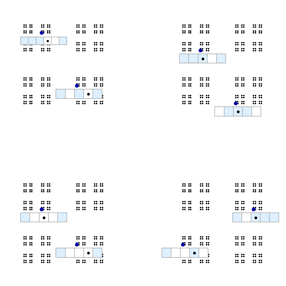
The key idea of this project is that the computation of a Turing machine is equivalent to a dynamical system in the Cantor set. Basically, each step of a computation is changing our tape of 0’s and 1’s to another different tape (while also shifting the position of the head). Therefore, using the language we have developed, each step of the Turing machine is mapping a point in the Cantor set into a different point.
In order to visualize this idea, we can see how the computing process of a complex Turing machine moves a point around the Cantor set:
In[]:=
turingtape=TuringMachine[{{1,0}->{4,0,1},{1,1}->{3,1,-1},{2,0}->{1,1,-1},{2,1}->{1,1,1},{3,0}->{1,1,1},{3,1}->{3,0,-1},{4,0}->{2,1,1},{4,1}->{2,1,1}},{1,{{},0}},200];LHStape=Table[turingtape[[All,2]][[i]][[1;;turingtape[[All,1]][[All,2]][[i]]-1]],{i,1,Length[turingtape]}];RHStape=Table[turingtape[[All,2]][[i]][[Max[1,turingtape[[All,1]][[All,2]][[i]]];;]],{i,1,Length[turingtape]}];
In[]:=
TMCantor=Table[Show[{ListPlot[PointsCantor,PlotStyle->Gray,AspectRatio->Automatic,PlotRange->{{-0.1,1.1},{-0.1,1.1}}],ListPlot[Table[CantorEmbedding[LHStape[[i]],RHStape[[i]]],{i,1,n}],PlotStyle->Directive[Darker[Blue],Opacity[0.5]],PlotMarkers->{Automatic,0.02}],If[n>1,(*ListLinePlot[Table[CantorEmbedding[LHStape[[i]],RHStape[[i]]],{i,n-1,n}],PlotStyle->Directive[Darker[Blue],Opacity[0.5]],PlotMarkers->{Automatic,0.02}]*)Graphics[{Blue,Arrow[Table[CantorEmbedding[LHStape[[i]],RHStape[[i]]],{i,n-1,n}]]}],Nothing]},Axes->False],{n,1,Length[turingtape]}];
vid4=FrameListVideo[TMCantor,FrameRate->5,VideoEncoding->"H264"];
In[]:=
cloudObj4=CloudExport[vid4,"MP4",Permissions->"Public"]
Out[]=
Our next step is to translate these discrete dynamics to smooth flows between two unit squares. The idea is to simulate with these flows the possible actions of a Turing machine: changing the position of the tape and rewriting a symbol; and apply them to all the points in the Cantor set which are affected by them.
One can check that these discrete dynamics acts on the regions that contain the Cantor set as piecewise linear functions, so we can implement the flows as some interpolations of these maps.
One can check that these discrete dynamics acts on the regions that contain the Cantor set as piecewise linear functions, so we can implement the flows as some interpolations of these maps.
For example, these are the flows that rewrite a 0 to a 1 and a 1 to a 0, respectively:
Out[]=

Out[]=

And these are the flows that correspond to shifting the tape to the right and to the left:
Out[]=

We can represent it as the following directed graph, where we have included an initializing state and a halting state:
The idea behind Topological Kleene Field Theories (TKFTs) is to thicken this graph, obtaining some “pipes” around each of the edges of the graph. This way, we can assign a unit square, and in particular a 2-dimensional Cantor set, to each of the nodes in the graphs. The computation of the Turing machine will be presented as a smooth flow between these squares. During this computation, the flow will “hit” different squares, each of them associated to the current head state of the Turing machine. The specific position in the square the flow goes through will encode the current state of the tape, using the embedding inside the Cantor set we described in the previous section.
An important remark to be made is that the topology of the manifold we construct plays an important role, and in general it must be nontrivial. This is caused by the fact that sometimes it is necessary to split a certain Cantor set into two branches that diverge, hence creating a nontrivial cobordism with holes in it. Indeed, one can check that the underlying graph that we use as the skeleton of our manifold is a strong deformation retract of the cobordism, so the homology invariants of the manifold, which we can interpret as its “topological complexity”, must be equal to those of the Turing machine graph.
Another important feature of this construction is that these flows are actually generated by a smooth vector field. In particular, this implies that no two trajectories cross each other. In practice, this implies that only reversible Turing machine can be simulated using this method. However, as explained in [2], this is not an actual limitation, as any Turing machine can be transformed into a reversible Turing machine by increasing the number of states.
Simulating any Turing machine
Simulating any Turing machine
Design of the flow
Design of the flow
Definitions pipe network
Definitions pipe network
Using these ideas we can define the functions to construct this pipe network which depends on the rules of our Turing machine.
Examples for different Turing machines
Examples for different Turing machines
Let us check now how the pipe system would like look for some Turing machines with a different number of states.
Let us start with a Turing machine with three states and the following rules:
Let us start with a Turing machine with three states and the following rules:
It is interesting to check that these rules (as all the rules presented in this work) represent indeed a reversible Turing machine.
Now we can see how the the cobordism for this rules looks like:
Now we can see how the the cobordism for this rules looks like:
We can choose another Turing machine with a greater number of states, in this case 6:
Then, we obtain the following more complex “pipe-system”:
Definitions of the Turing machine
Definitions of the Turing machine
Now that we understand the idea of this construction and computed the graphics for our simulation, we can define the functions that will actually simulate any (reversible) Turing machine.
We start by defining the expressions for the flow
Definitions of the flow
Definitions of the flow
We will define a flow that leaves a state a proceed with a transition of the Turing machine. Therefore, it will depend on the state it leaves and the one it goes to, the new symbol that it writes and the shift it performs. A halting condition is also included, which computes the flow from the particular state to the halting state.
Now we are ready to define the function that simulates any Turing machine.
Simulations
Simulations
After all this discussion, we are ready to simulate any reversible Turing machine.
For example, we can start with the following Turing machine:
Then, the simulation we get for these rules is the following:
We can try another Turing machine with different number of states:
The simulation we get for this case is the following:
Concluding Remarks
Concluding Remarks
This project has fully realized Topological Kleene Field Theory as a framework for simulating computation through smooth dynamical systems. By encoding the simulations of any Turing machine as explicit computational flows, we have demonstrated how discrete symbolic computation can be reinterpreted in terms of smooth flows, explicitly showing their Turing completeness. The fact that we can embed any computation into cobordisms and extract its dynamics through flows suggests a promising research direction at the intersection of dynamical systems, category theory, and theoretical computer science.
There is important room for future work. It would be interesting to further understand and visualize the structure of the vector fields associated with the flows. Another next step into developing the theoretical framework would be to analyze the dynamics for points outside the Cantor set, and explore if they can be used to improve the computations. Finally, it would be interesting to explore ideas on how to embed computations into other continuous dynamical systems, and use this property to better understand both, the dynamics of the system and the computations we can reproduce on it.
There is important room for future work. It would be interesting to further understand and visualize the structure of the vector fields associated with the flows. Another next step into developing the theoretical framework would be to analyze the dynamics for points outside the Cantor set, and explore if they can be used to improve the computations. Finally, it would be interesting to explore ideas on how to embed computations into other continuous dynamical systems, and use this property to better understand both, the dynamics of the system and the computations we can reproduce on it.
Acknowledgments
Acknowledgments
◼
To Ángel González-Prieto, Eva Miranda ad Daniel Peralta-Salas, who have supported me enormously, believing in me and giving me incredible opportunities during the last few years.
◼
To Stephen Wolfram, for the wonderful conversations about my project and his priceless suggestions on how to approach and improve this exposition of TKFTs. In particular, for suggesting taking this path of simulating any arbitrarily large Turing machine instead of taking the less practical and not so useful approach of simulating a reversible universal Turing machine.
◼
To my mentor during the Wolfram Summer School, Dugan Hammock, for all his help during the beginning of this project at the Wolfram Summer School.
The project that gave rise to these results received the support of a fellowship from the “la Caixa” Foundation (ID 100010434). The fellowship code is LCF/BQ/PFA25/11000070.
This article has been partially supported by the project reference PID2023-146936NB-I00 financed by the Spanish State Agency MCIN/AEI/10.13039/501100011033/ FEDER, UE.
This article has been partially supported by the project reference PID2023-146936NB-I00 financed by the Spanish State Agency MCIN/AEI/10.13039/501100011033/ FEDER, UE.
References
References
1
.C. Moore (1990), “Unpredictability and undecidability in dynamical systems”, Physical Review Letters. https://sites.santafe.edu/~moore/nonlinearity-gs.pdf
2
.Á. González-Prieto, E. Miranda and D. Peralta-Salas (2025), “Topological Kleene Field Theories: A new model of computation”, Preprint arxiv. https://arxiv.org/abs/2503.16100
3
.I. Ramos (2025), “Computation trough smooth dynamics: simulating TKFT’s”, Wolfram Community https://community.wolfram.com/groups/-/m/t/2959123
4
.CITE THIS NOTEBOOK
CITE THIS NOTEBOOK
Turing completeness through smooth dynamics: expanding simulations of TKFT’s
by Isaac Ramos
Wolfram Community, STAFF PICKS, November 5, 2025
https://community.wolfram.com/groups/-/m/t/3570717
by Isaac Ramos
Wolfram Community, STAFF PICKS, November 5, 2025
https://community.wolfram.com/groups/-/m/t/3570717