We consider a single quantum particle in the Anderson tight-binding model. This is a simple model for the motion of a quantum particle, such as an electron, and it is generally studied on a lattice. The model exhibits two kinds of behavior, which roughly correspond to those of a conductor, where the particle propagates freely through the material, and those of an insulator, where the particle is localized to a particular spot in the material.
We start by assuming that we have lattice and that we have a different quantum state corresponding to the particle sitting on each of these lattice sites, . In this basis, the Hamiltonian for the system is given by
N
sites
1,2,...,N
|1〉,|2〉,...,|N〉
H=diag(,,...,)-tA
ϵ
1
ϵ
2
ϵ
N
where ,,..., are the “mean field” energies of each lattice site, is the “hopping parameter,” and is the adjacency matrix of the graph describing the system (e.g., a regular lattice). The values of will ultimately control whether the system behaves as a conductor or an insulator.
ϵ
1
ϵ
2
ϵ
N
t>0
A
ϵ
i
One familiar example for the adjacency matrix is
A
A
i,j
δ
i,j+1
δ
i+1,j
which describes a 1D lattice with open boundary conditions.
In[]:=
Graph[Table[ii+1,{i,1,10}]]
Out[]=

The term in the Hamiltonian will then describe the transition amplitude for the particle to hop from one site on the lattice to an adjacent site. If we further assume that ==...==ϵ, meaning that there is simply a fixed energy associated with the particle sitting on any given lattice site, we recover the standard 1D tight-binding model from condensed matter physics, which has (discretized) plane waves for eigenstates. (For a nice introduction to the tight binding model in 1D, see David Tong’s lecture notes on Applications of Quantum Mechanics: https://www.damtp.cam.ac.uk/user/tong/aqm.html.)
-tA
ϵ
1
ϵ
2
ϵ
N
In[]:=
(*Numberoflatticesites*)=50;(*Adjacencymatrix*)A=Table[N[KroneckerDelta[i,j+1]+KroneckerDelta[i+1,j]],{i,},{j,}];(*On-siteenergy*)ϵ=2.0;(*HoppingStrength*)t=1.0;(*Hamiltonianfor1Dtight-bindingmodel*)Htb1d=ϵIdentityMatrix[]-t*A;
(*Plotafeweigenstates*)ListLinePlot[Abs@Eigenvectors[Htb1d][[1;;3]],Frame->True,FrameLabel->Map[Style[#,Black,20]&,{"n","|ψ(n)|"}],AspectRatio->0.8,PlotMarkers->{Automatic,10}]
Out[]=
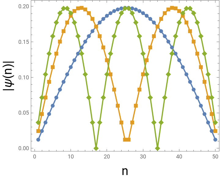
However, in real materials, there will be many electrons interacting with one another, potentially in a highly complex manner. One way to try to account for the effects of these complex interactions is to modify the energy associated with the particle sitting on a given lattice site, , and to approximate it as simply a random number. This is the claim that the “mean field” experienced by the particle at that site is “disordered.” If each is a random variable drawn from an interval , we now have the Anderson tight-binding model.
ϵ
i
ϵ
i
[-W/2,W/2],W>0
The eigenstates of this system are qualitatively different in character: rather than being freely propagating plane waves, they instead exhibit “Anderson localization,” meaning that they are localized around a small number of lattice points, for sufficiently strong disorder.
In[]:=
W=10.0;Hal1d=DiagonalMatrix[RandomReal[{-W/2,W/2},]]-t*A;
In[]:=
ListLinePlot[Abs@Eigenvectors[Hal1d][[1;;8]],Frame->True,FrameLabel->Map[Style[#,Black,20]&,{"n","|ψ(n)|"}],AspectRatio->0.8,PlotMarkers->{Automatic,10},PlotRange->All]
Out[]=
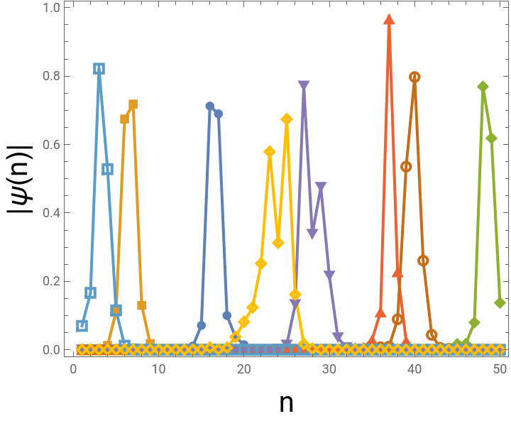
Anderson localization, and its many-body physics generalization, is a topic of active research in modern condensed matter physics.
For the problem we consider today, we will use another adjacency matrix, this time not associated with a 1D lattice, but rather associated with an Erdos-Renyi random graph, , a graph with vertices, in which each pair of vertices , with , is connected by an edge with probability and is left unconnected with probability . In others words,
G(N,p)
N
(i,j)
i<j
p
1-p
A
i,j
A
j,i
0ifi=j |
1withprobabilityp |
0withprobability1-p. |
We depict a few Erdos-Renyi random graphs below.
In[]:=
GenERAdjMat[n_,p_]:=Block[{adjMat,e},adjMat=ConstantArray[0,{n,n}];Do[If[RandomChoice[{p,1-p}->{1,0}]==1,adjMat[[i,j]]=1;adjMat[[j,i]]=1;],{i,1,n-1},{j,i+1,n}];adjMat]
In[]:=
GraphicsRow[AdjacencyGraph[GenERAdjMat[15,#],GraphLayout->"CircularEmbedding"]&/@{0.1,0.3,0.5,1.0}]
Out[]=
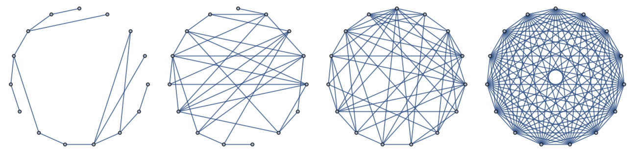
This model of a random graph is interesting because it exhibits a connectivity/percolation phase transition as we vary (source: Networks, Mark Newman). Specifically, when , a so-called “giant component” forms in the graph, meaning that one set of connected vertices contains nodes, , such that in the limit , an infinite cluster is formed in the graph and contains a finite fraction of all nodes.We now investigate the ground state properties of the Anderson tight binding Hamiltonian on an Erdos-Renyi random graph as we vary through . Specifically, we are interested in the degree of localization of the single-particle ground state, which we capture through the inverse participation ratio (IPR) That the IPR captures the degree of localization of the wave function can be seen through two limiting examples. If we have a completely spread out state, with a normalized wave function given simply by , then , and the IPR is a small number. On the other hand, if we have a totally localized wave function on our lattice, , then . For states of intermediate localization, the values of the IPR will fall between and 1.
p
p>=1/(N-1)
p
c
SN
0<S<1
N->∞
S
p
p
c
IPR(ψ)=ψ(i)
∑
i
4
|
ψ=1
N
IPR(ψ)=1/N
ψ=
δ
i,
i
0
IPR(ψ)=1
1/N
We now calculate the IPR for the ground state of our system for two cases, one where =...==0<->W=0, which describes pure hopping on the random graph, and one with significant disorder
ϵ
1
ϵ
N
W/t=10.
Out[]=
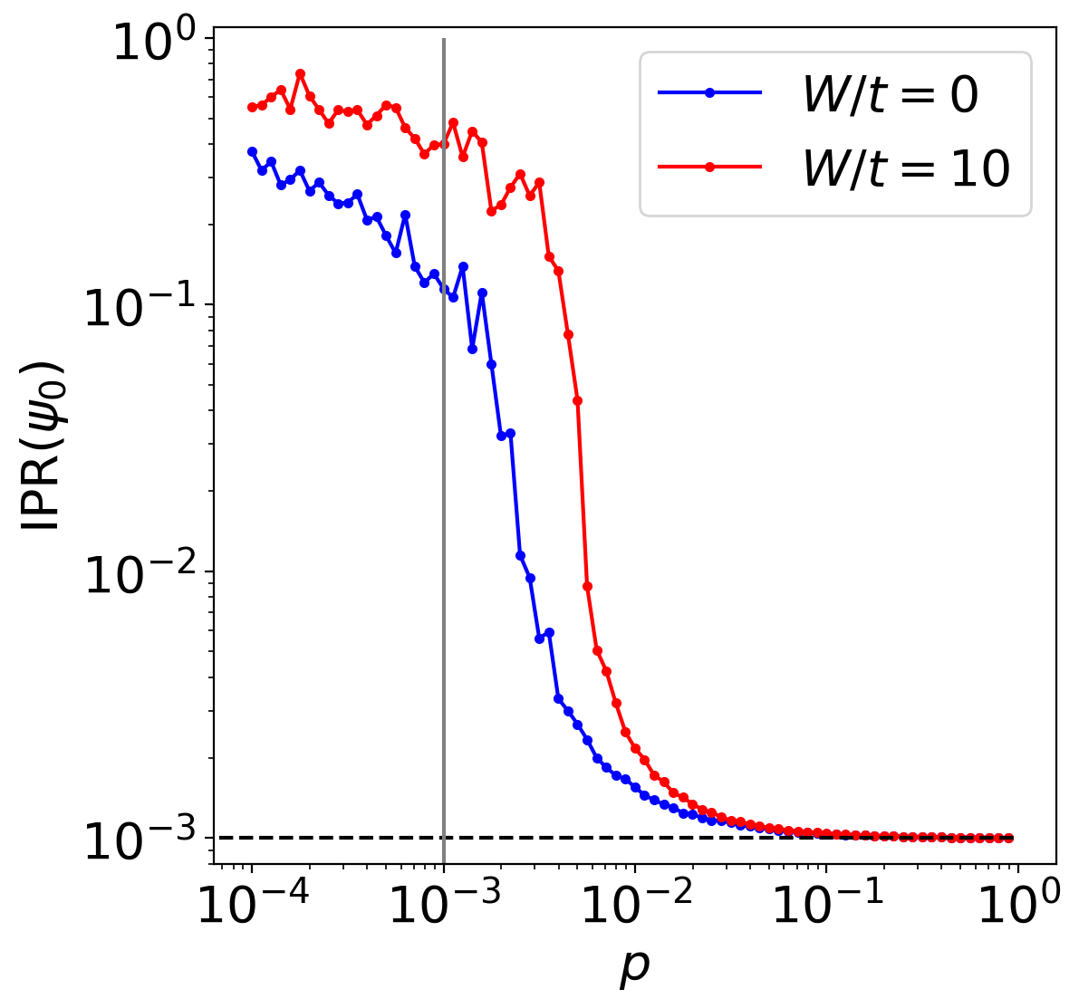
In this figure, the percolation transition threshold is indicated by the vertical gray line, and the fully delocalized IPR value of is indicated by the horizontal black dashed line. The results in the figure were obtained on random graphs with nodes, where the disorder is fixed as we vary , and each curve is averaged over three manifestations of random graphs .
IPR=1/N
N=1000
p
A(p)
We see that for networks with a high degree of connectivity (higher ), the IPR is low, meaning that eigenstates delocalize. Indeed, for , we have a complete graph, meaning that the adjacency matrix is constant (apart from the diagonal).
p
p=1
In[]:=
GenERAdjMat[10,1.0]//MatrixForm
Out[]//MatrixForm=
0 | 1 | 1 | 1 | 1 | 1 | 1 | 1 | 1 | 1 |
1 | 0 | 1 | 1 | 1 | 1 | 1 | 1 | 1 | 1 |
1 | 1 | 0 | 1 | 1 | 1 | 1 | 1 | 1 | 1 |
1 | 1 | 1 | 0 | 1 | 1 | 1 | 1 | 1 | 1 |
1 | 1 | 1 | 1 | 0 | 1 | 1 | 1 | 1 | 1 |
1 | 1 | 1 | 1 | 1 | 0 | 1 | 1 | 1 | 1 |
1 | 1 | 1 | 1 | 1 | 1 | 0 | 1 | 1 | 1 |
1 | 1 | 1 | 1 | 1 | 1 | 1 | 0 | 1 | 1 |
1 | 1 | 1 | 1 | 1 | 1 | 1 | 1 | 0 | 1 |
1 | 1 | 1 | 1 | 1 | 1 | 1 | 1 | 1 | 0 |
One encounters Hamiltonians of this form elsewhere in physics, and their ground state is known to be delocalized. For example, an important problem in the theory of superconductivity involves two particles interacting via a short-range attractive interaction above a filled Fermi sea. This is known as the “Cooper problem,” and the Hamiltonian in second quantization is given by
which has eigenstates
is known as a “Cooper pair,” and it plays a central role in the theory of superconductivity due to Bardeen, Cooper, and Schrieffer (BCS).
our Hamiltonian without a disordered mean field has a very similar spectrum to the Cooper problem Hamiltonian.
CITE THIS NOTEBOOK
CITE THIS NOTEBOOK
Ground state properties of the Anderson tight-binding model on an Erdos-Renyi random graph
by Matthew Kafker
Wolfram Community, STAFF PICKS, August 10, 2025
https://community.wolfram.com/groups/-/m/t/3528022
by Matthew Kafker
Wolfram Community, STAFF PICKS, August 10, 2025
https://community.wolfram.com/groups/-/m/t/3528022