Sundaresan-Krishnaswamy Technique for Estimation of Process Parameters
Authors: Housam Binous and Ahmed Bellagi
Sundaresan-Krishnaswamy Technique for Estimation of Process Parameters
Authors: Housam Binous and Ahmed Bellagi
Authors: Housam Binous and Ahmed Bellagi
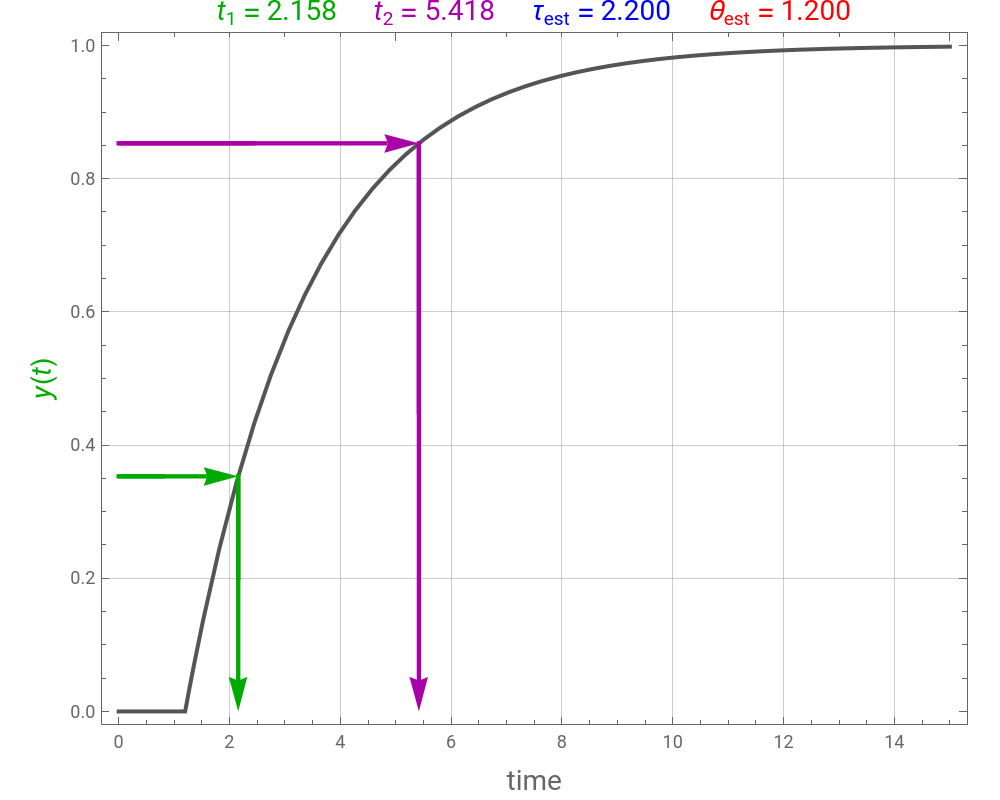
Consider a first-order plus delay model defined by the transfer function , where , , and are the gain, time constant, and time delay, respectively. In order to find and , Sundaresan and Krishnaswamy [1, 2] use the normalized response of the model to a step-forcing function: at two different times, and . These times are selected such that the normalized response reaches 35.3% at and 85.3% at . The recipe gives the estimated values of the time constant and delay time by =0.674803(–) and =1.29382–0.293815.We plot the normalized response for user-set values of and . Perfect agreement is observed between the estimated values and and actual values (taken equal to: and ).
G(s)=
K
-θs
e
τs+1
K
τ
θ
τ
θ
y
KM
U(s)=M/s
t
1
t
2
t
1
t
2
τ
est
t
2
t
1
θ
est
t
1
t
2
τ
θ
τ
est
θ
est
τ=2.2
θ=1.2
References :
[1] K. R. Sundaresan and P. R. Krishnaswamy, “Estimation of Time Delay Time Constant Parameters in Time, Frequency, and Laplace Domains,” The Canadian Journal of Chemical Engineering, 56(2), 1978 pp. 257–262. doi:10.1002/cjce.5450560215.
[2] D. E. Seborg, T. F. Edgar, D. A. Mellichamp, and F. J. Doyle III, Process Dynamics and Control, 4th ed., New York: Wiley, 2017.
We set the values of and .
τ=2.2
θ=1.2
In[]:=
θ=1.2;(*timedelayθ*)τ=2.2;(*timeconstantτ*)
In[]:=
y[t_]:=InverseLaplaceTransform[1/sExp[-θs]1/(τs+1),s,t];
We find and .
t
1
t
2
sol1=FindRoot[y[t]0.353,{t,τ+θ}];(*timesuchthatnormalizedresponsereaches35.3%*)sol2=FindRoot[y[t]0.853,{t,2τ+θ}];(*timesuchthatnormalizedresponsereaches85.3%*)
In[]:=
t1=t/.sol1
Out[]=
2.1579
In[]:=
t2=t/.sol2
Out[]=
5.41811
In[]:=
Show[Plot[y[t],{t,0,15},AspectRatio0.8,GridLinesAutomatic,FrameTrue,ImageSize400{1.25,1},PlotStyle{Darker@Gray,Thick},PlotRange{-0.02,1.02},FrameLabel{Style["time",14],Style[Row[{Style["y",Italic],"(",Style["t",Italic],")"}],14,Darker@Green]},PlotLabelRow[{Style[" = ",Darker@Green,14],Style[NumberForm[t1,{4,3}],14,Darker@Green]," ",Style[" = ",Darker@Magenta,14],Style[NumberForm[t2,{4,3}],14,Darker@Magenta]," ",Style[" = ",Blue,14],Style[NumberForm[0.674803(t2-t1),{4,3}],14,Blue]," ",Style[" = ",Red,14],Style[NumberForm[1.29382t1-0.293815t2,{4,3}],14,Red]}]],Graphics[{Darker@Green,Thickness[0.005],Arrow[{{t1,0.353},{t1,0}}],Arrow[{{0,0.353},{t1,0.353}}],Darker@Magenta,Thickness[0.005],Arrow[{{t2,0.853},{t2,0}}],Arrow[{{0,0.853},{t2,0.853}}]}]]
t
1
t
2
τ
est
θ
est
Out[]=