Wolfram Cloud Document

The Wolfram Emerging Leaders Program: High School (WELP:HS) is a remote, semester-long program designed for exceptional graduates from the Wolfram High School Summer Research Program to continue to develop their skills. Students work in a small group over the course of a semester to do either a research-based project or a product development–based project under the guidance of expert mentors. Projects are centered around a topic at the intersection of the group’s interests.

This essay was written by:

◼

Eric Archerman

◼

Niko Moustakas

◼

Max Grunwald

In nature, systems of coupled oscillators, which are oscillators that affect each other’s movement, tend to synchronize. In addition to systems of simple physical oscillators such as coupled springs or two pendulum clocks hanging from the same beam, this synchronization affect turns up in the flashing of fireflies, in the firing of heart cells, and when crowds clap. To model these phenomena, Yoshiki Kuramoto introduced the Kuramoto Model in 1975. Compared to previous models for synchronization, the Kuramoto Model’s advantage is that it uses the relative phase angles instead of the discrete states of the oscillators. The Kuramoto Model has been shown to accurately describe a coupled system’s behavior for some cases, and in this paper, we apply the model to others systems such as groups of fireflies. In addition to physical applications, we also explore theoretical implementations, such as the Kuramoto model over non-global topologies as well as the change in behavior as the coupling varies over space. Finally, we further the work of Yoshiki Kuramoto by finding the limit of how synchronized any given system can be through an analysis of the order parameter.

Background

The Kuramoto Model, introduced by Yoshiki Kuramoto in 1975 [4], is a popular model for characterizing the synchronization of coupled oscillators (oscillators that affect each other’s movement). In many fields such as biology, physics, and electromagnetics, oscillators trend towards synchronization, some examples of which are below.

In this section, we will rebuild the Kuramoto Model from scratch for an intuitive understanding in the later sections.

A Mathematical Oscillator

A verbal definition for an oscillator is an object that follows a certain path of motion repetitively in the same manner. Mathematically, if we describe the position of our oscillator in an

dimensional space as

X(t)=(

(t),

(t),...,

(t))

, then we have that

X(t)=X(t+p)

for some period

[2]. From this definition of our oscillator, we know that the motion of our oscillator through space will be some sort of twisted loop. Below is an example for an oscillator in a 3 - dimensional space.

In[]:=

points=RandomReal[{-0.1,0.1},{6,3}];curve=BSplineCurve[points,SplineDegree->2,SplineClosed->True];frames=Table[Graphics3D[{curve,Red,PointSize[0.02],Point[BSplineFunction[points,SplineDegree->2,SplineClosed->True][t]]},Boxed->True],{t,1,0,-0.01}];ListAnimate[frames,AnimationRunning->False]

Out[]=

Our oscillator’s path through space is basically a glorified loop, which means that we can map the oscillator’s path onto the unit circle. Think of it like untangling the loop and then scaling that to fit the unit circle. And just as the red dot in the graph above represents our oscillator’s movement through space, we can add a red dot to represent the oscillator on our unit circle. Note that this step abstracts the geometry of our oscillator away so that we only think about its position relative to its path.

In[]:=

frames2=Table[Graphics[{Circle[],Red,PointSize[0.02],Point[{Cos[theta],Sin[theta]}]},PlotRange->{{-1.5,1.5},{-1.5,1.5}},ImageSize->150],{theta,0,2Pi,0.06283185307}];Row[{ListAnimate[frames,AnimationRunning->False],ListAnimate[frames2,AnimationRunning->False]}]

Out[]=

So when we work with oscillators, we can just work with the abstracted unit circle, and when we want more oscillators, we just add more dots to the unit circle. An important concept for this definition of an oscillator is phase angles, which gives the moving dot some meaning. We define the phase angle as the angle formed by the positive x-axis and the line between the origin and the red dot. This mean that our phase angle

θ∈[0,2π)

, which is the range of our phase function

θ(t)

. The limited range means we must be careful when we do arithmetic, as we have to take everything

mod2π

. Furthermore, we consider the dot’s speed (without external influences)



ω

around the unit circle to be its natural frequency. So knowing our oscillator’s behavior without external forces, and our next challenge is to model how our oscillator behaves when interacting with another one.

Two Oscillators

We now explore the behavior of two coupled oscillators. When our two oscillators

are not coupled with





and





, their behavior will look something like the subsequent animation.

listFrames=Table[Graphics[{Thick,Circle[],Red,PointSize[Large],Point[{Cos[angle],Sin[angle]}],Text[Subscript[θ,1],{Cos[angle],Sin[angle]},{0,1.5}],Blue,PointSize[Large],Point[{Cos[1.15*(angle+π/3)],Sin[1.15*(angle+π/3)]}],Text[Subscript[θ,2],{Cos[1.15*(angle+π/3)],Sin[1.15*(angle+π/3)]},{0,-1.5}]}],{angle,0,2π,0.1}];ListAnimate[listFrames,ImageSize->300,AnimationRunning->False]

Out[]=

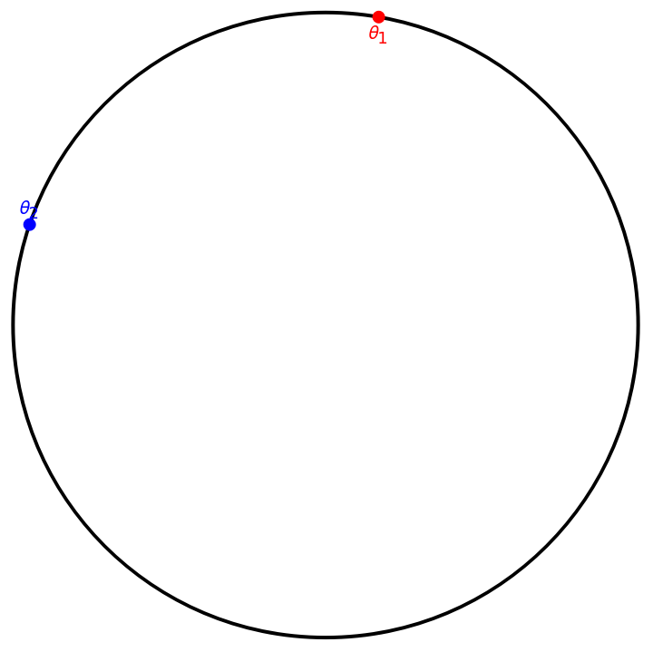
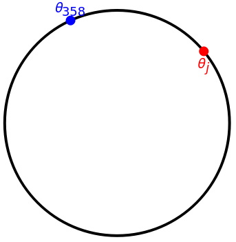
However, when the two oscillators, are coupled, they will influence each other’s motion because they will exert forces on each other, the extent to which we can write as

f



. This means that with coupled oscillators, we’ll have





+f(

)

and





+f(

In reality though, the actual values of

and

shouldn’t affect

, but instead it should be the relationship between the two phase angles, so we revise

f



, the force exerted on

, to

f



. We arbitrarily choose

and not

because it’s arbitrary so we can choose

accordingly. This gives us that





+f(

)

and





+f(

Now that we have our equations for



and



set up, our next step is to find some equation to model our function

. We try to construct a rough graph, starting with thinking about critical values. When

, we’ll have that the phases of the oscillators, are the same, resulting in no force between the two oscillators. Thus

f(0)=0

. When

<π

, our phases will look something like the below.

angle=0.69;Graphics[{Thick,Circle[],Red,PointSize[Large],Point[{Cos[angle],Sin[angle]}],Text[Subscript[θ,j],{Cos[angle],Sin[angle]},{0,1.5}],Blue,PointSize[Large],Point[{Cos[1.15*(angle+π/3)],Sin[1.15*(angle+π/3)]}],Text[Subscript[θ,i],{Cos[1.15*(angle+π/3)],Sin[1.15*(angle+π/3)]},{0,-1.5}]}]

Out[]=

Many Oscillators

Extending our formula for two oscillators to many oscillators is actually quite simple if we just consider the pairwise interactions between all oscillators. So then our formula becomes

The Order Parameter

Before we write a Mathematica implementation for the model, it will be useful to develop a more sophisticated measure for synchronicity, as well as a nice way to visualize the state of the system. As previously discussed, the complex path taken by the oscillators through N-space can be simply viewed as a path around a unit circle, and the position of each oscillator can be defined by its phase angle along the circle. So given some list of phases, we can create a nice visualization of the points that looks something like this:

A very important thing we can do now is to look at the centroid of these points- that is, their average position. Drawing a vector from the origin to the centroid will give us a really nice measure of the global state of the system. Many mathematical analyses of the Kuramoto model begin here [4]; we will use this as a nice visualization function. The magnitude of this vector will reflect the total synchronicity of the system. If all the points are about equally distributed, the centroid will be near the origin, with a magnitude of near zero; if they are all bunched together, the centroid will be close to the edge of the circle, with a magnitude of near one. Convention is to use complex numbers instead of vectors for this process, as Euler’s formula makes the math very nice and simple.

The following functions calculate the order parameter and the magnitude r of the order parameter:

Consider the following synchronized and unsynchronized systems:

Look at their differences in synchronicity:

Equally valuable will be a way to visualize the system with its order parameter, given below:

Let’s look at each of the given systems with this function

We can also bring time into this model, and create an animation representing the evolving state of the system over time. The following function creates such an animation. It takes a function object which itself inputs a number (t) and outputs a vector (θ), as well as an ending time for the animation. It distributes the points slightly off of the unit circle for clarity.

The order parameter jumps around a bit, but it stays near the origin. (Note: We recommend the reader delete output cells for the animations after running, so as not to strain computer resources). We can write a function to get the average value of r for large values of t:

For a fully synchronized system, this limit should be pretty close to 1. Let’s see if that’s the case...

Implementation and Exploration

Implementation at Last

This is actually quite simple. Mathematica allows us to pretty easily implement the Kuramoto model using NDSolve. The following function takes two equally sized lists ω and ϕ representing the natural frequencies and initial phases respectively of the oscillators of the system. κ represents the coupling constant; for now κ will be a simple scalar value. The function will return a key containing interpolation function objects for each oscillator.

Let’s try it out for a 100-oscillator system. We begin by defining the parameters of the system.

We don’t technically have to choose our natural frequencies from a normal distribution, but its more realistic to how synchronization occurs in the natural world. Initial phase is a totally random property with no default value, and we expect it to be about evenly distributed over the interval [-π, π]. Natural frequency, however, is an innate and non-arbitrary property of an individual, so we expect the distribution of this trait in a natural population to be approximately normal. We also chose to have the mean natural frequency at 1 instead of 0. This will help to illustrate a point later.

We now run the model to get our solution.

First, lets just look at a plot of our phases over time:

Notice that the plot seems to bifurcate into multiple regions of stability. As discussed earlier, this is because we are dealing in modulo 2π- each of those regions will be in the same place on the unit circle. Let’s look at the rotator for this simulation. We need to quickly define a getKeyFunc function which translates the key into a function admissible by the rotatorPlot.

Sure enough, we see that the points cluster together. This is synchronization in action; all modes of synchronization which obey Kuramoto’s assumptions will cohere in a manner similar to what was just shown. To confirm, lets look at the magnitude of the order parameter for large t.

Watch the rotator model again, but imagine that you yourself begin rotating in unison with the oscillators, so that from your vantage point they appear stationary. This is the essence of the transition to a stationary reference frame. If we rotate at the right speed (choose Ω correctly) and the right time (choose ψ correctly) we can make the average speed of rotation appear to be 0 and make all the oscillators converge on a phase θ = 0.

Let’s rerun our rotator, but this time after transitioning to a rotational frame of reference.

Non-Global Topologies

Introduction

Plotting its adjacency matrix gives

The following function implements the Kuramoto Model for a non-global system. It takes the additional argument of an adjacency matrix representing the system topology- notice the a[[i,j]] factor in the sum.

High deg

To begin testing this function, lets consider a specific family of graphs studied in detail by Stephen Strogatz [14]. He describes his findings in detail in this video, and his papers are included in our references. Strogatz was studying n-vertex graphs in which each vertex was connected to a certain number of its nearest neighbors. These graphs are called circulant. Following Strogatz, we will label this the degree deg. He claims that as long as each vertex is connected to at least 78.89% of the rest of the system (that is to say, deg > 0.7889 (n - 1)), the system will be capable of synchrony. Let’s test this idea.

We’ll begin by writing a function which will return the neighbor graph with n vertices and degree deg. Note that in practice, when deg is odd, each vertex will connect with deg + 1 other vertices, which is just a natural product of the way the network is set up.

We want the adjacency matrix of this graph. Due to the way Mathematica indexes vertices, we’ll need to reshuffle the adjacency matrix somewhat for our model to work.

Now we’ll implement synchronization. We’ve chosen the use a higher standard deviation for ω because it will help to illustrate the point; but note that the synchronicity in this section will be lower than those in the previous one.

However, we will now get our key from kuramotoAdjacency, with the extra matrix argument:

Let’s jump straight into the rotator plot for our oscillators.

The problem with this visualization method now is that it is too abstract; it doesn’t let us see what is going on at the local level. We want to know how the non-global topology impacts synchronization. Let’s create a new visualization function, called topologyPlot, which lets us see things more clearly. This plot takes a list of interpolating functions as opposed to an NDSolve key because of compiler difficulties presumably related to aliasing. This plot will represent phase with color. A phase of 0 is red; as the phase increases, the hue turns orange, then green, then turquoise. A phase of π is blue. The hue then turns purple, then magenta, and finally returns to red at 2π.

Let’s look at the synchronicity limit for this system- we can see it gets highly synchronized.

If you watch it slowly, its possible to see that certain areas synchronize with each other before the whole system coheres. This behavior will become yet more apparent in the sections to come.

Low deg

Let’s now look at a system which will not synchronize. We will still deal with circulant graphs, but this time we will use a degree of 2.

At a glance, the graph looks extremely sparse.

Let’s run the model and to check that it does not in fact synchronize.

We can see from the rotator that the system never achieves synchronicity; the small number of oscillators makes it prone to random fluctuation, but by and large r remains small.

On the topology plot we can see that locally some areas seem to synchronize briefly, but it never becomes a global phenomenon.

Finally, lets look at the synchronicity limit.

Random graphs

Another extremely important kind of topology to consider is that of a randomly generated system. The perfect symmetry discussed above is unlikely in nature; what happens when we just start throwing things together ad hoc? We will consider graphs of n vertices and e random connections between these vertices. e must be a number between 0 and n(n-1)/2. To begin, consider a large e. In this case, we chose e = 2500, which for 50 vertices means that we have about 50% connectivity.

Let’s create our graph with these specifications. We will array it in a circle just like the last section.

The graph certainly appears suitably random. Will it synchronize?

We’re going to ignore the visualizations here and jump straight to the synchronicity limit.

Synchronization is definitely occurring. Finally, let’s consider random graphs with low connectivity. We won’t dwell too long on this, because it’s pretty obvious what will happen.

e = 500 represents only about 10% connectivity, which should not be enough to achieve significant coherence.

Let’s run the model and see what happens:

As expected, synchronization does not occur.

Coupling Over Space

Let’s specifically define the coupling matrix κ that we will be using

If that explanation didn’t make sense, imagine we’re basically doing the same thing we did in the previous section, but instead of a simple adjacency matrix we use an interaction matrix where the value of the (i,j)’th square represents the coupling strength between oscillators i and j. The κ matrix we have just generated is plotted below, though due to how the squares have to be stretched out into a line it isn’t intuitively obvious why it should look like this.

Perhaps a better way to visualize what is going on is to draw a line between each pair of oscillators, where the thickness of the line represents the coupling strength. Fortuitously, this is actually very visually clear.

Let’s now implement the Kuramoto model on this setup.

Let’s check out the rotator plot to confirm that synchronization is occurring.

Again we run into a visualization problem, because that rotator model gives no clue as to how spacial location plays a role in synchronization. To remedy this, we will create a spacialPlot function which represents each of the oscillators as squares in a grid as we have been doing previously. Color will represent phase, in the same way as with the topologyPlot function.

Now we can watch as our oscillator grid synchronizes:

We can actually see coherence spread across the grid like a fungus. We can make it look even cooler by transitioning to a rotational frame.

This will eliminate the visual noise of the rapidly shifting technicolor grid, letting us more easily watch the oscillators synchronise. The authors also elected not to correct for phase shift, because we think the different colors are fun.

Much future work is necessary in this area, but the cursory results given here are really cool.

Modeling Firefly Synchronization

Introduction to firefly synchronization

Kuramoto model implementation

This function models a static n by n array of fireflies, simulating a field of stationary fireflies all visible to each other. In this model, each firefly has a intrinsic flashing frequency (ω) and initial phase (ϕ) randomly assigned from a biologically relevant distribution. Each pair of fireflies has a coupling constant (κ), which depends on the distance between the pair using a switching function. If the distance is greater than the signaling radius (rad), the coupling constant is set to 0, otherwise the coupling constant is a set value (κ0). The examples in this chapter use this function to simulate a field of 15x15 fireflies, for different values of κ0 and rad.

Running and visualizing a simulation

Here we simulate a population of 225 fireflies in a 15x15 grid. Using arbitrary values for the coupling constant (κ0) and signaling radius (rad). This simulation runs from 0 to 400π seconds.

This plot shows each oscillator as a cosine function for the first 10π seconds of the simulation. At the beginning of the simulation, all the oscillators have a different period and phase, resulting in no synchronization. Fairly quickly we can observe that the oscillators start to synchronize into a common period although they are still somewhat out of phase.

This animation shows the same data for the 225 fireflies visually as a grid of blinking squares, and it illustrates how rapidly the fireflies sync in the simulation with these parameters.

This plot shows each oscillator as a cosine function for the last 10π seconds of the simulation. Here we can see that the oscillators’ periods and phases appear tightly synchronized at the end of the simulation, although they are not perfectly in phase.

This animation illustrates how synchronized the fireflies remain at the end of the simulation

Quantifying the synchronization over time

To quantify the synchronization of fireflies in this simulation I computed all the pairwise correlations between the fireflies over a sliding window of time. The average correlation is reported for each point in time.

This expression below applies the windowAvgCorrelation function defined above to the simulation data between 0 and 100π seconds.

These expressions set the proper x and y axes label values for the plot

Plotting the average pairwise correlation coefficient over time for the example simulation. This demonstrates that for the parameters that I chose the system reaches its maximum correlation very rapidly and remains correlated for the length of the simulation

Initial exploration of model sensitivity to the coupling constant and signaling radius

We were interested to see how the different parameters like the coupling constant and signaling radius affect the synchronization in the simulation. Here we rerun the simulation with a weaker coupling constant (0.5 instead of 0.75 previously)and a shorter signaling radius (8 instead of 10 previously), which should increase the amount of time to achieve maximum synchronization.

Plotting the average pairwise correlation coefficient over time for the example simulation. This demonstrates that for the new parameters that I chose the system reaches a lower maximum correlation and takes longer to achieve steady state compared to the first simulation. We were surprised that the simulation plateaued at a lower maximum correlation!

This plot reveals two key differences between the simulations. It reveals that the coupling constant and signaling radius both affect the maximum correlation achieved and the time to reach steady state.

Systematic exploration of the effects of the coupling constant and signaling radius on the maximum correlation

Clearly we need to examine how changing both the coupling constant and signaling radius simultaneously affect the synchronization of a set of fireflies.This code systematically scans combinations of κ0 and rad values, and runs a simulation for each combination. By computing the maximum correlation of each simulation at steady state, we can understand how the coupling constant and the signaling radius determine the maximum correlation of each system.

The expression above explores κ0 between 0.2 and 1.0, and rad between 2 and 22. Since this expression takes approximately an hour to run we've pasted the output below

Visualization

Here we manipulate the data from all the simulations in the scan in order to enable a heat map visualization at the end of this section.

dataSet2 contains the extracted maximum correlation values of each simulation.

Here we use a wrapping function to convert the 1D list (dataSet2) into a 2D table.

This gives the correct tick marks for the y axis of the heat map.

This gives the correct tick marks for the x axis of the heat map.

This heat map shows the landscape of the maximum correlation as a function of both coupling strength and signaling radius.

There are several conclusions we can reach by examining this heat map. The first is that below a critical value of the signaling radius of 4-5, it is impossible for the fireflies to synchronize regardless of the value of the coupling constant. The second is that beyond the minimum/critical signaling radius, the effect of a smaller signaling radius can be offset by a stronger coupling constant, and vice versa.

References & Future Work

Future Work

References

[1] Buck, J., Buck, E. (1976). Synchronous Fireflies. Scientific American, 234(5), 74–85. doi:10.1038/scientificamerican0576-74

[2] Brockmann, Dirk (2023) Introduction to Complex Systems: The Kuramoto Model. (https://rocs.hu-berlin.de/courses/complex-systems/script/kuramoto-model/)

[3 ] Channel, C. (2018). Stefano Ruffo - Statistical physics of the Kuramoto model [YouTube Video]. In YouTube. https://www.youtube.com/watch?v=glb_OvWhP2A&list=PLhHzlh0skeGKuR_j3dhPmGY9aFp_sb5Q4

[4] Daniels, Bryan C. (2005) Synchronization of Globally Coupled Nonlinear Oscillators: the Rich Behavior of the Kuramoto Model.

[5] Ermentrout, G . B . (1991) An adaptive model for synchrony in the firefly Pteroptyx malaccae . J. Math. Biol. 29, 571

[6] Guo, Y., Zhang, D., Li, Z., Wang, Q., & Yu, D. (2021). Overviews on the applications of the Kuramoto model in modern power system analysis. International Journal of Electrical Power & Energy Systems, 129, 106804. doi:10.1016/j.ijepes.2021.106804

[7] Kotwal, T., Jiang, X., & Abrams, D.M. (2017). Connecting the Kuramoto Model and the Chimera State. Physical review letters, 119 26, 264101 .

[8] Mirollo, R. E., and Strogatz, S. H. (1990) Synchronization of pulse-coupled biological oscillators. SIAM J. Appl. Math. 50, 1645.

[9] Pikovskij, A., Rosenblum, M., & Kurths, J. (2007a). Synchronization: A universal concept in Nonlinear Sciences. Cambridge Univ. Press.

[10] Ramírez-Ávila, G. M., Kurths, J., Depickère, S., Deneubourg, J.-L. (2018) Modeling Fireflies Synchronization. Nonlinear Systems and Complexity, 131–156.

[11] Ride my Kuramotocycle. (2018, April 14). Ride my Kuramotocycle! Complexity-Explorables.org. https://www.complexity-explorables.org/explorables/ride-my-kuramotocycle/

[12] Sokol, J. (2022) How Do Fireflies Flash in Sync? Studies Suggest a New Answer. (https://www.quantamagazine.org/how-do-fireflies-flash-in-sync-studies-suggest-a-new-answer-20220920/)

[13] Strogatz, S. (2000) Nonlinear Dynamics and Chaos: With Applications to Physics, Biology, Chemistry and Engineering, Westview Press, 105-108

[14] Townsend, A., Stillman, M.E., & Strogatz, S.H. (2019). Circulant networks of identical Kuramoto oscillators: Seeking dense networks that do not globally synchronize and sparse ones that do. arXiv: Adaptation and Self-Organizing Systems.

[15] Trees, B. R., Saranathan, V., & Stroud, D. (2005). Synchronization in disordered Josephson junction arrays: Small-world connections and the Kuramoto model. Physical Review E, 71(1). doi:10.1103/physreve.71.016215

CITE THIS NOTEBOOK

Theoretical and Applied Analyses of the Kuramoto Model
by Wolfram Emerging Leaders Program
Wolfram Community, STAFF PICKS, January 18, 2024
https://community.wolfram.com/groups/-/m/t/3105614