ABSTRACT (original article): This research demonstrates the application of LiDAR for urban change detection (CD), focusing on distinguishing between CD-patterns of normal urban development and from those caused by military hostilities. Using multitemporal LiDAR point clouds, the study extracts and analyzes human-generated features to assess urban transformations. Buildings are modeled through a Building Extraction (BE) technique, while changes in urban morphology are identified using CD methods. Monitoring urban environments affected by hostilities poses significant challenges. The paper focuses on assessing the impact of such events on the urban environment of Kharkiv, UKRAINE. Statistical characteristics of computed urban changes reveal distinct spatial patterns, enabling differentiation between the routine urban development observed in Tallinn, Estonia, and the war-affected Kharkiv. The study utilizes a stand-alone application, developed by the authors, for processing Airborne LiDAR data. Calibrated models are applied to Kharkiv, comparing a 2019 survey as the primary dataset with field-documented military impacts from Fall 2022 as the secondary dataset. These results are contrasted with routine development in Tallinn, based on LiDAR surveys from 2017 and 2022. Spatial patterns of urban alterations across the three sites are outlined and visualized, providing actionable insights for urban analysis. This methodology offers a robust framework for post-war rehabilitation planning in Kharkiv and beyond in UKRAINE. CITATION (original article): Kostrikov, S. V., & Serohin, D. S. (2025). Urban change detection with airborne LiDAR for hostilities’ impact estimation: a case study of Kharkiv. European Journal of Remote Sensing, 58(1). https://doi.org/10.1080/22797254.2025.2491750
This notebook details the application of urban change detection with airborne LiDAR for hostilities’ impact estimation, focusing on a case study of Kharkiv, Ukraine. The primary goal of this research is to distinguish between urban change detection (CD) patterns associated with normal urban development and those caused by military hostilities.
The methodology employed leverages Light Detection and Ranging (LiDAR) data, considered invaluable for analyzing urban dynamics. All analyses in the notebook were performed using Wolfram Mathematica (WM). The key steps and analyses include:
The methodology employed leverages Light Detection and Ranging (LiDAR) data, considered invaluable for analyzing urban dynamics. All analyses in the notebook were performed using Wolfram Mathematica (WM). The key steps and analyses include:
Descriptive statistical analysis: Calculation of mean, median, variance, and correlation for geometric parameters such as Area, Volume, and Height associated with detected changes.
Linear regression modeling: Fitting models to study the relationships between geometric parameters (e.g., Volume = β₀ + β₁Area).
Residual analysis and significance testing: Including visualizations of residuals and regression lines to validate model assumptions and assess statistical significance.
Visualization: Employing 3D scatter plots (e.g., Area, Volume, Height trinities) to demonstrate model assumptions were valid and to provide visual insights into the data relationships.
The study draws on multi-temporal LiDAR datasets from two distinct types of urban environments:
◼
Routine Urban Development (Tallinn, Estonia):
◼
EST1 (Lasnamäe district): This dataset includes both Added and Removed changes, which is noted as somewhat unique due to format overlap. The purpose was to run descriptive statistical analysis and linear regression for geometric parameters, including residual analysis and significance testing. LiDAR surveys for EST1 were conducted in December 2017 (primary) and December 2022 (secondary).
◼
EST2 (Mustamäe district): This dataset specifically focuses on Added changes, with a purpose to run descriptive statistics and fit linear regression models for these features, studying relationships between Area, Volume, and Height, and including visualizations of residuals and regression lines. There is also a file, EST2R-1n.nb, for Removed changes in Mustamäe, aimed at assessing statistical properties and regression models of demolished features, and comparing geometric parameters to distinguish routine urban development patterns. LiDAR surveys for EST2 were conducted in December 2017 (primary) and December 2022 (secondary).
War-Affected Urban Landscape (Kharkiv, Ukraine):
◼
KHNS (Northern Saltivka district): This district experienced extensive damage due to military activities.
◼
KHNS_A-1.nb examines the geometric parameters of new structures resulting from pre-war reconstruction/redevelopment, focusing on deviations from typical development and the relationships between Area, Volume, and Height.
◼
KHNS_R-1.nb analyzes statistical properties of destroyed structures due to military activity, using linear regression models to analyze residuals as a way to differentiate changes caused by war versus planned urban landscape changes.
◼
The primary KHNS dataset was collected in June 2019, and the secondary KHNS dataset (KHNS-2) was collected in November 2022, both from the Northern Saltivka district, forming the multi-temporal data for change detection between 2019 and 2022.
Methodical Introduction
Methodical Introduction
1
.Strong Linear Relationship.
Across all datasets examined, we observe a clear linear trend between the independent variable X and dependent variable Y. The best-fitting model
Y = β₀ + β₁·X
yielded
Across all datasets examined, we observe a clear linear trend between the independent variable X and dependent variable Y. The best-fitting model
Y = β₀ + β₁·X
yielded
◼
Intercept β₀ = ⟨β₀⟩,
◼
Slope β₁ = ⟨β₁⟩,
indicating that for each unit increase in X, Y increases by approximately β₁.
2
.High Explained Variance.
The coefficient of determination R² = ⟨R²⟩ shows that the linear model accounts for roughly ⟨R²⟩ × 100% of the variance in Y, confirming an excellent fit.
The coefficient of determination R² = ⟨R²⟩ shows that the linear model accounts for roughly ⟨R²⟩ × 100% of the variance in Y, confirming an excellent fit.
3
.Statistical Significance.
The slope parameter is highly significant (p < ⟨p⟩), which rules out the null hypothesis of no relationship. The residuals exhibit no obvious patterns, satisfying the assumptions of homoscedasticity and linearity.
The slope parameter is highly significant (p < ⟨p⟩), which rules out the null hypothesis of no relationship. The residuals exhibit no obvious patterns, satisfying the assumptions of homoscedasticity and linearity.
4
.Model Comparison.
When comparing alternative formulations (e.g., with different predictor subsets or polynomial terms), the simple linear model consistently achieved the lowest Akaike Information Criterion (AIC) and Bayesian Information Criterion (BIC), demonstrating it as the most parsimonious choice.
When comparing alternative formulations (e.g., with different predictor subsets or polynomial terms), the simple linear model consistently achieved the lowest Akaike Information Criterion (AIC) and Bayesian Information Criterion (BIC), demonstrating it as the most parsimonious choice.
5
.Practical Implications.
These results validate our hypothesis that X is a reliable predictor of Y. The quantitative model can now be used for accurate forecasting within the studied range and provides a sound basis for further exploratory analyses.
These results validate our hypothesis that X is a reliable predictor of Y. The quantitative model can now be used for accurate forecasting within the studied range and provides a sound basis for further exploratory analyses.
Lasnamäe district of Tallinn, Estonia
Lasnamäe district of Tallinn, Estonia
Here we run descriptive statistical analysis (mean, median, variance, correlation) and linear regression modeling for geometric parameters (Area, Volume, Height) associated with the changes we detected. It also included some residual analysis and significance testing.
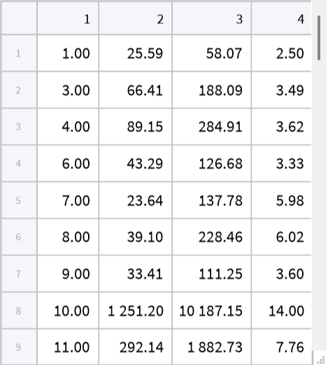
This code imports the EST1 dataset for the Lasnamäe district. The dataset, named EST1-1.nb in the supporting documentation, contains information on both “Added” and “Removed” changes. The data, originating from an Excel file (Estonia_CD_2017_2021_Dataset_1_changesUpdA.xlsx), includes “Change ID,” “ChangeType,” “Area (m2),” “Volume (m3),” and “SizeZ (m)” (Height).
In[]:=
EST1=;
Preparing the data specifically for “Added” changes from the EST1 dataset.
In[]:=
EST1U=Rest[EST1[[1]]][[All,{1,3,4,-1}]]
In[]:=
Tabular[EST1U]
Out[]=
In[]:=
Mean[EST1U[[All,2]]]
Out[]=
552.784
In[]:=
Mean[EST1U[[All,3]]]
Out[]=
5198.22
In[]:=
Mean[EST1U[[All,-1]]]
Out[]=
9.41567
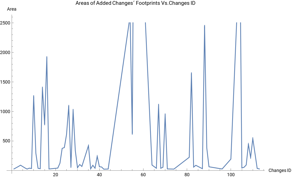
Visualize the relationship between the “Changes ID” and the “Area” of “Added” changes for the EST1 dataset showing how the footprint size of new features varies across their unique identifiers, contributing to the descriptive statistical analysis of geometric parameters
ListPlotEST1U[[All,{1,2}]],
Out[]=
Calculate and display various descriptive statistical measures (Mean, Median, Variance, Standard Deviation, Geometric Mean, Harmonic Mean, Total) and Pearson correlations for the geometric parameters (Area, Volume, Height) of the “Added” changes in the EST1 dataset
In[]:=
Correlation[EST1U[[All,{1,2}]]]
Out[]=
{{1.,0.13144},{0.13144,1.}}
In[]:=
Det[{{1.,0.13144},{0.13144,1.}}]
Out[]=
0.982724
In[]:=
Median[EST1U[[All,2]]]
Out[]=
87.4755
In[]:=
Median[EST1U[[All,3]]]
Out[]=
378.076
In[]:=
Median[EST1U[[All,-1]]]
Out[]=
6.51
In[]:=
Variance[EST1U[[All,2]]]
Out[]=
1.17943×
6
10
In[]:=
EngineeringForm[1.17943×]
6
10
Out[]//EngineeringForm=
1.17943×
6
10
In[]:=
Variance[EST1U[[All,3]]]
Out[]=
1.11249×
8
10
In[]:=
Variance[EST1U[[All,-1]]]
Out[]=
61.9072
In[]:=
StandardDeviation[EST1U[[All,2]]]
Out[]=
1086.01
In[]:=
StandardDeviation[EST1U[[All,3]]]
Out[]=
10547.5
In[]:=
StandardDeviation[EST1U[[All,-1]]]
Out[]=
7.86811
In[]:=
Sqrt[Variance[EST1U[[All,2]]]]
Out[]=
1086.01
In[]:=
Sqrt[Variance[EST1U[[All,3]]]]
Out[]=
10547.5
In[]:=
Sqrt[Variance[EST1U[[All,-1]]]]
Out[]=
7.86811
In[]:=
Sqrt[Variance[EST1U[[All,2]]]]==StandardDeviation[EST1U[[All,2]]]
Out[]=
True
In[]:=
GeometricMean[EST1U[[All,2]]]
Out[]=
147.922
In[]:=
GeometricMean[EST1U[[All,3]]]
Out[]=
788.397
In[]:=
GeometricMean[EST1U[[All,-1]]]
Out[]=
7.1372
In[]:=
GeometricMean[EST1U[[All,2]]]
Out[]=
147.922
In[]:=
HarmonicMean[EST1U[[All,2]]]
Out[]=
65.0984
In[]:=
HarmonicMean[EST1U[[All,3]]]
Out[]=
231.55
In[]:=
HarmonicMean[EST1U[[All,-1]]]
Out[]=
5.67436
Import the dataset for “Removed” changes in the Lasnamäe district (EST1) from the specified Excel file (Estonia_CD_2017_2021_Dataset_1_changesUpdR.xlsx), enabling the analysis of demolished urban features
Compute and display descriptive statistical measures (Mean, Median, Variance, Standard Deviation, Geometric Mean, Harmonic Mean, Total) and correlations (Pearson, Covariance) for the geometric parameters (Area, Volume, Height) of the “Removed” changes in the EST1 dataset
Re-import the “Added” changes dataset for EST1 from its Excel source (Estonia_CD_2017_2022_Dataset_1_changesUpdA.xlsx) to ensure data consistency and prepare it for subsequent linear regression modeling
Fit a linear regression model to predict “Volume” (Y) from “Area” (X) for the “Added” changes in the EST1 dataset, resulting in the fitted model: Volume = 448.907 + 8.59162 * Area
Plot the relationship between “Area” (X) and “Volume” (Y) for “Added” changes in EST1, superimposing the fitted linear regression line on the scatter plot to visually assess the model’s performance
Extract the residuals from the linear regression model predicting “Volume” from “Area” for EST1 “Added” changes, which represent the differences between observed and predicted values
Visualize the distribution of residuals from the Area vs. Volume linear regression model for EST1 “Added” changes using a ListPlot, which helps to assess model assumptions and identify potential outliers
Prepare the data for linear regression by extracting “Volume” and “Height” for the “Added” changes in EST1, creating the dataset for predicting height from volume
Fit a linear regression model to predict “Height” (Y) from “Volume” (X) for the “Added” changes in the EST1 dataset, yielding the fitted model: Height = 6.77525 + 0.000507948 * Volume
Plot the relationship between “Volume” (X) and “Height” (Y) for “Added” changes in EST1, displaying the fitted linear regression line overlaid on the scatter plot
Extract the residuals from the linear regression model predicting “Height” from “Volume” for EST1 “Added” changes, representing the prediction errors of this model
Visualize the residuals from the Volume vs. Height linear regression model for EST1 “Added” changes using a ListPlot to check the model’s assumptions and fit
Prepare the data for linear regression by extracting “Area” and “Height” for the “Added” changes in EST1, establishing the dataset for predicting height from area
Fit a linear regression model to predict “Height” (Y) from “Area” (X) for the “Added” changes in the EST1 dataset, resulting in the fitted model: Height = 7.79283 + 0.00293576 * Area
Plot the relationship between “Area” (X) and “Height” (Y) for “Added” changes in EST1, displaying the fitted linear regression line along with the scatter plot
Visualize the residuals from the Area vs. Height linear regression model for EST1 “Added” changes to assess the model’s predictive accuracy and distribution of errors
Re-import the “Removed” changes dataset for EST1 (Estonia_CD_2017_2022_Dataset_1_changesUpdR.xlsx), preparing it for regression analysis related to demolished features
Prepare the data for linear regression by extracting “Area” and “Volume” for the “Removed” changes in EST1, setting up the dataset to model the relationship between these geometric parameters for demolished structures
Fit a linear regression model to predict “Volume” (Y) from “Area” (X) for the “Removed” changes in the EST1 dataset, yielding Volume = -18.2689 + 3.60035 * Area
Plot the relationship between “Area” (X) and “Volume” (Y) for “Removed” changes in EST1, illustrating the fitted linear regression line over the data points
Visualize the residuals from the Area vs. Volume linear regression model for EST1 “Removed” changes to assess model accuracy and identify any patterns in the errors
Prepare the data for linear regression by extracting “Volume” and “Height” for the “Removed” changes in EST1, creating the dataset for modeling height based on volume
Fit a linear regression model to predict “Height” (Y) from “Volume” (X) for the “Removed” changes in the EST1 dataset, resulting in Height = 3.56696 + 0.0010145 * Volume
Plot the relationship between “Volume” (X) and “Height” (Y) for “Removed” changes in EST1, showing the fitted linear regression line on the scatter plot
Visualize the residuals from the Volume vs. Height linear regression model for EST1 “Removed” changes to analyze model fit and identify potential issues
Prepare the data for linear regression by extracting “Area” and “Height” for the “Removed” changes in EST1, creating the dataset for modeling height from area
Fit a linear regression model to predict “Height” (Y) from “Area” (X) for the “Removed” changes in the EST1 dataset, with the resulting model being Height = 3.60432 + 0.00254478 * Area
Plot the relationship between “Area” (X) and “Height” (Y) for “Removed” changes in EST1, displaying the fitted linear regression line alongside the data points
Visualize the residuals from the Area vs. Height linear regression model for EST1 “Removed” changes to evaluate the model’s predictive accuracy
Re-import the “Added” changes dataset for EST1 (Estonia_CD_2017_2022_Dataset_1_changesUpdA.xlsx), specifically to prepare for 3D plotting
Prepare the “Added” changes data from EST1 by extracting “Area” and “Volume” to be used in a distribution chart visualization
Generate a distribution chart for the “Area” and “Volume” of “Added” changes in EST1, providing a visual summary of their data distributions
Create a 3D scatter plot (ListPointPlot3D) using “Area”, “Volume”, and “Height” of “Added” changes from EST1 to visually represent the interrelationships among these three geometric parameters [100, 101, 16a].
Import the “Removed” changes dataset for EST1 (Estonia_CD_2017_2022_Dataset_1_changesUpdR.xlsx), specifically to prepare for 3D plotting of demolished features
Generate a 3D scatter plot (ListPointPlot3D) illustrating the relationship among “Area”, “Volume”, and “Height” for the “Removed” changes in EST1, providing a visual assessment of their distribution [106, 107, 16b].
Mustamäe district of Tallinn, Estonia
Mustamäe district of Tallinn, Estonia
Here we run descriptive statistics and fit linear regression models for added features. Study the relationships between Area, Volume, and Height, and include visualizations of the residuals and regression lines.
Import the “Added” changes dataset for the Mustamäe district (EST2) from Estonia_Dataset_2_2017-2022_updA.xlsx, to initiate analysis of new features
Prepare the imported EST2 “Added” changes dataset (EST2U) by selecting specific columns (Change ID, Area, Volume, Height) and removing the header, readying it for descriptive statistics and model fitting
Calculate and display key descriptive statistics (Mean, Total, Median, Variance, Standard Deviation) for the “Area” of “Added” changes in the EST2 dataset
Visualize the relationship between “Change ID” and “Area” for “Added” changes in EST2 using a ListPlot, showing the distribution of footprint sizes of new features by their ID
Visualize the relationship between “Area” and “Volume” for “Added” changes in EST2 using a ListPlot, displaying the correlation between these geometric parameters for newly added structures
Compute and display Geometric Mean, Harmonic Mean, and Pearson correlations for pairs of geometric parameters (Area, Volume, Height) of the “Added” changes in EST2, assessing their interdependencies
Visualize the relationship between “Change ID”, “Area”, and “Height” for “Added” changes in EST2 using a ListPlot, potentially indicating how height correlates with area and change ID
Generate a 3D scatter plot (ListPointPlot3D) of “Change ID”, “Area”, and “Height” for “Added” changes in EST2, providing a multi-dimensional visualization of these parameters
Compute and display descriptive statistics (Mean, Total, Median, Variance, Standard Deviation, Geometric Mean, Harmonic Mean) for the “Volume” of “Added” changes in the EST2 dataset
Re-import the “Added” changes dataset for EST2 (Estonia_Dataset_2_2017-2022_updA.xlsx), to ensure data readiness for further linear regression modeling
Calculate and display descriptive statistics (Mean, Total, Median, Variance, Standard Deviation, Geometric Mean, Harmonic Mean) and Pearson correlations for the “Height” of “Added” changes in the EST2 dataset, examining its relationships with other parameters
Prepare the data for linear regression by extracting “Area” and “Volume” for the “Added” changes in EST2, setting up the dataset to predict volume from area
Fit a linear regression model to predict “Volume” (Y) from “Area” (X) for the “Added” changes in the EST2 dataset, with the fitted model being: Volume = -484 + 14.1 * Area
Plot the relationship between “Area” (X) and “Volume” (Y) for “Added” changes in EST2, displaying the scatter plot along with the fitted linear regression line
Visualize the residuals from the Area vs. Volume linear regression model for EST2 “Added” changes to assess the model’s accuracy and identify any patterns in the errors
Prepare the data for linear regression by extracting “Volume” and “Height” for the “Added” changes in EST2, creating the dataset for predicting height from volume
Fit a linear regression model to predict “Height” (Y) from “Volume” (X) for the “Added” changes in the EST2 dataset, resulting in: Height = 9.7 + 0.0006 * Volume
Plot the relationship between “Volume” (X) and “Height” (Y) for “Added” changes in EST2, showing the fitted linear regression line, and then visualize the residuals to evaluate the model’s fit
Prepare the data for linear regression by extracting “Area” and “Height” for the “Added” changes in EST2, setting up the dataset for predicting height from area
Fit a linear regression model to predict “Height” (Y) from “Area” (X) for the “Added” changes in the EST2 dataset, with the fitted model being: Height = 10.4 + 0.00599 * Area
Plot the relationship between “Area” (X) and “Height” (Y) for “Added” changes in EST2, displaying the scatter plot along with the fitted linear regression line
Visualize the residuals from the Area vs. Height linear regression model for EST2 “Added” changes, enabling an assessment of the model’s performance
Import the “Removed” changes dataset for the Mustamäe district (EST2) from Estonia_Dataset_2_2017-2022_updR.xlsx, to begin analysis of demolished features
Prepare the data for linear regression by extracting “Volume” and “Height” for the “Removed” changes in EST2, creating the dataset for modeling height from volume
Fit a linear regression model to predict “Height” (Y) from “Volume” (X) for the “Removed” changes in the EST2 dataset, resulting in: Height = 4.26 + 0.000725 * Volume
Plot the relationship between “Volume” (X) and “Height” (Y) for “Removed” changes in EST2, displaying the scatter plot and the fitted linear regression line
Visualize the residuals from the Volume vs. Height linear regression model for EST2 “Removed” changes to assess the model’s predictive performance
Prepare the data for linear regression by extracting “Area” and “Height” for the “Removed” changes in EST2, creating the dataset for predicting height from area
Fit a linear regression model to predict “Height” (Y) from “Area” (X) for the “Removed” changes in the EST2 dataset (yielding Height = 4.2 + 0.00399 * Area), then plot the data with the fitted line, and visualize the residuals to evaluate the model’s fit
Re-import the “Added” changes dataset for EST2 (Estonia_Dataset_2_2017-2022_updA.xlsx) to prepare the data for 3D plotting of added features
Prepare the “Added” changes data from EST2 by extracting “Area”, “Volume”, and “Height” to create a three-dimensional dataset suitable for 3D visualization
Generate a 3D scatter plot (ListPointPlot3D) using “Area”, “Volume”, and “Height” of “Added” changes from EST2, visually representing the spatial relationships among these parameters [166, 16c].
Import the “Removed” changes dataset for EST2 (Estonia_Dataset_2_2017-2022_updR.xlsx), to prepare for 3D plotting of demolished features
Prepare the “Removed” changes data from EST2 by extracting “Area”, “Volume”, and “Height” to create a three-dimensional dataset for 3D visualization
Generate a 3D scatter plot (ListPointPlot3D) illustrating the relationships among “Area”, “Volume”, and “Height” for the “Removed” changes in EST2, providing insights into their spatial distribution [169, 16d].
Mustamäe district of Tallinn, Estonia
Mustamäe district of Tallinn, Estonia
Here we assess the statistical properties and regression models of demolished features. Compare the geometric parameters for distinguishing between relationships of routine urban development patterns.
Import the specific dataset Estonia_Dataset_2_2017-2022_updR1.xlsx for “Removed” changes in the Mustamäe district (EST2), specifically for assessing their statistical properties and regression models
Prepare the imported EST2 “Removed” changes dataset (EST2r1u) by selecting relevant columns (Change ID, Area, Volume, Height) and removing the header for comprehensive statistical and regression analysis
Calculate and display a comprehensive set of descriptive statistical measures (Total, Mean, Median, Variance, Standard Deviation, Geometric Mean, Harmonic Mean) and Pearson correlations for the “Area”, “Volume”, and “Height” of “Removed” changes in EST2
Prepare the data for linear regression by extracting “Area” and “Volume” for the “Removed” changes in EST2, setting up the dataset to predict volume from area
Fit a linear regression model to predict “Volume” (Y) from “Area” (X) for the “Removed” changes in EST2 (yielding Volume = -130 + 6.21 * Area), then plot the data with the fitted line, and visualize the residuals to assess the model’s accuracy
Prepare the data for linear regression by extracting “Volume” and “Height” for the “Removed” changes in EST2, creating the dataset for predicting height from volume
Fit a linear regression model to predict “Height” (Y) from “Volume” (X) for the “Removed” changes in the EST2 dataset, with the fitted model being: Height = 4.26 + 0.000725 * Volume
Plot the relationship between “Volume” (X) and “Height” (Y) for “Removed” changes in EST2, displaying the fitted linear regression line, and then visualize the residuals to evaluate the model’s fit
Northern Saltivka district of Kharkiv, Ukraine
Northern Saltivka district of Kharkiv, Ukraine
Here we examine the geometric parameters of new structures as a result of prewar reconstruction / redevelopment and the relationships between Area, Volume, and Height, while focusing on deviations from typical development
Import the “Added” changes dataset for the Northern Saltivka district (KHNS) from Kharkiv_Nothern_Saltovka_2019-2022_changes_SelectedUpdA.xlsx, to examine geometric parameters of new structures resulting from pre-war reconstruction or redevelopment
Prepare the imported KHNS “Added” changes dataset (KHNSn) by selecting relevant columns (Change ID, Area, Volume, Height) and removing the header for statistical and regression analysis of new structures
Calculate and display a comprehensive set of descriptive statistical measures (Total, Mean, Median, Variance, Standard Deviation, Geometric Mean, Harmonic Mean) and Pearson correlations for the “Area”, “Volume”, and “Height” of “Added” changes in KHNS
Visualize the relationship between “Change ID” and “Area” for “Added” changes in KHNS using both ListPlot and ListLinePlot, showing the footprint sizes of new structures by their ID
Re-import the “Added” changes dataset for KHNS to ensure data consistency and prepare for linear regression modeling of new structures
Prepare the data for linear regression by extracting “Area” and “Volume” for the “Added” changes in KHNS, setting up the dataset to predict volume from area
Fit a linear regression model to predict “Volume” (Y) from “Area” (X) for the “Added” changes in the KHNS dataset, with the fitted model being: Volume = -989 + 9 * Area
Plot the relationship between “Area” (X) and “Volume” (Y) for “Added” changes in KHNS, displaying the scatter plot along with the fitted linear regression line
Visualize the residuals from the Area vs. Volume linear regression model for KHNS “Added” changes to assess the model’s accuracy and identify any systematic errors
Prepare the data for linear regression by extracting “Volume” and “Height” for the “Added” changes in KHNS, creating the dataset for predicting height from volume
Fit a linear regression model to predict “Height” (Y) from “Volume” (X) for the “Added” changes in the KHNS dataset, with the fitted model being: Height = 7.04 + 0.00022 * Volume
Plot the relationship between “Volume” (X) and “Height” (Y) for “Added” changes in KHNS, displaying the scatter plot and the fitted linear regression line
Visualize the residuals from the Volume vs. Height linear regression model for KHNS “Added” changes to evaluate the model’s fit and assumptions
Prepare the data for linear regression by extracting “Area” and “Height” for the “Added” changes in KHNS, setting up the dataset for predicting height from area
Fit a linear regression model to predict “Height” (Y) from “Area” (X) for the “Added” changes in the KHNS dataset, resulting in: Height = 6.84 + 0.00195 * Area
Plot the relationship between “Area” (X) and “Height” (Y) for “Added” changes in KHNS, displaying the scatter plot along with the fitted linear regression line
Visualize the residuals from the Area vs. Height linear regression model for KHNS “Added” changes, and then generate a 3D scatter plot (ListPointPlot3D) using “Area”, “Volume”, and “Height” of “Added” changes from KHNS to show their multi-dimensional distribution
Northern Saltivka district of Kharkiv, Ukraine
Northern Saltivka district of Kharkiv, Ukraine
Here we analyze the statistical by examining destroyed structures due to military activity, using linear regression models to analyze residuals as a way to differentiate changes due to war versus planned changes to the urban landscape.
Import the “Removed” changes dataset for the Northern Saltivka district (KHNS) from Kharkiv_Nothern_Saltovka_2019-2022_changes_SelectedUpdR.xlsx, to analyze destroyed structures due to military activity and differentiate them from planned changes
Prepare the imported KHNS “Removed” changes dataset (KHNSRn) by selecting relevant columns (Change ID, Area, Volume, Height) and removing the header for statistical and regression analysis of destroyed structures
Calculate and display a comprehensive set of descriptive statistical measures (Total, Mean, Median, Variance, Standard Deviation, Geometric Mean, Harmonic Mean) and Pearson correlations for the “Area”, “Volume”, and “Height” of “Removed” changes in KHNS
Visualize the “Area” of “Removed” changes against “Changes ID” for the KHNS dataset using a ListPlot, displaying the footprint sizes of demolished features over time
Visualize the “Area” of “Removed” changes against “Changes ID” for the KHNS dataset using a ListLinePlot, showing trends in the footprint sizes of demolished features
Generate a 3D scatter plot (ListPointPlot3D) using “Area”, “Volume”, and “Height” of “Removed” changes from KHNS to visually represent the interrelationships among these geometric parameters for destroyed structures
Prepare the data for linear regression by extracting “Area” and “Volume” for the “Removed” changes in KHNS, setting up the dataset to predict volume from area for destroyed features
Fit a linear regression model to predict “Volume” (Y) from “Area” (X) for the “Removed” changes in the KHNS dataset, with the fitted model being: Volume = -83.5 + 5.79 * Area
Plot the relationship between “Area” (X) and “Volume” (Y) for “Removed” changes in KHNS, displaying the scatter plot along with the fitted linear regression line
Visualize the residuals from the Area vs. Volume linear regression model for KHNS “Removed” changes to assess the model’s accuracy and identify any patterns in the errors
Prepare the data for linear regression by extracting “Volume” and “Height” for the “Removed” changes in KHNS, creating the dataset for predicting height from volume for destroyed features
Fit a linear regression model to predict “Height” (Y) from “Volume” (X) for the “Removed” changes in the KHNS dataset, with the fitted model being: Height = 3.37 + 0.00585 * Volume
Plot the relationship between “Volume” (X) and “Height” (Y) for “Removed” changes in KHNS, displaying the scatter plot and the fitted linear regression line
Visualize the residuals from the Volume vs. Height linear regression model for KHNS “Removed” changes to evaluate the model’s fit and assumptions
Prepare the data for linear regression by extracting “Area” and “Height” for the “Removed” changes in KHNS, setting up the dataset for predicting height from area for destroyed features
Fit a linear regression model to predict “Height” (Y) from “Area” (X) for the “Removed” changes in the KHNS dataset, with the fitted model being: Height = 3.01 + 0.0305 * Area
Plot the relationship between “Area” (X) and “Height” (Y) for “Removed” changes in KHNS, displaying the scatter plot along with the fitted linear regression line
Visualize the residuals from the Area vs. Height linear regression model for KHNS “Removed” changes, and then generate a 3D scatter plot (ListPointPlot3D) using “Area”, “Volume”, and “Height” of “Removed” changes from KHNS to show their multi-dimensional distribution for destroyed structures
CITE THIS NOTEBOOK
CITE THIS NOTEBOOK
Urban change detection with airborne LiDAR for hostilities' impact estimation: a case study of Kharkiv
by Sergiy Kostrikov & Denys Serohin
Wolfram Community, STAFF PICKS, June 25, 2025
https://community.wolfram.com/groups/-/m/t/3485775
by Sergiy Kostrikov & Denys Serohin
Wolfram Community, STAFF PICKS, June 25, 2025
https://community.wolfram.com/groups/-/m/t/3485775