Chapter 5 Problem 51: Rolf Winter’s problem
Chapter 5 Problem 51: Rolf Winter’s problem
This notebook calculates the “exponential” decay of a state without perturbation theory
This notebook calculates the “exponential” decay of a state without perturbation theory
In[]:=
Remove["Global`*"]

Write down the solution, Equation (1) in Rolf Winter’s article
In[]:=
fFunc=HeavisideTheta[x]GSin[q]Sin[lq];
In[]:=
intg=Sqrt[2/a]2nExp[-ITq^2]qSin[q](qSin[q(l+1)]+f)/((q^2-Pi^2n^2)(q^2+GqSin[2q]+G^2Sin[q]^2));
Aaron’s suggestion: Change variables to integrate over a finite range
In[]:=
qu=u/(1-u);qJac=D[qu,u];
Calculate the probability that the particle is inside the well as a function of time. This should resemble Figure 2 from Rolf’s paper, so use those parameters.
In[]:=
Ts={0,0.01,0.025,0.05,0.075,0.1,0.2,0.3,0.4,0.5,1,2,4,6,8,8.25,8.5,8.75,9,9.125,9.25,9.375,9.5,9.625,9.75,9.875,10,10.25,10.5,10.75};
In[]:=
vals={a1,n1,G6};
In[]:=
t1=AbsoluteTime[];ψ=NIntegrate[(qJacintg)/.qqu/.vals/.f0/.TTs,{u,0,1},{l,-1,0},PrecisionGoal4];t2=AbsoluteTime[];
In[]:=
(t2-t1)/60
Out[]=
4.66643958
In[]:=
ρ=Conjugate[ψ]ψ;
In[]:=
ρPlot=Transpose[{Ts,Re[ρ]}];
In[]:=
ρPlot
Out[]=
{{0,0.810615},{0.01,0.814405},{0.025,0.818401},{0.05,0.834619},{0.075,0.786283},{0.1,0.738178},{0.2,0.641932},{0.3,0.569031},{0.4,0.485395},{0.5,0.413617},{1,0.189909},{2,0.0404815},{4,0.00180554},{6,0.0000831278},{8,3.65764×},{8.25,2.36829×},{8.5,1.81344×},{8.75,1.1998×},{9,7.03745×},{9.125,6.03456×},{9.25,5.54757×},{9.375,4.98301×},{9.5,4.07987×},{9.625,3.01049×},{9.75,2.13864×},{9.875,1.68756×},{10,1.58604×},{10.25,1.41513×},{10.5,7.12582×},{10.75,4.04842×}}
-6
10
-6
10
-6
10
-6
10
-7
10
-7
10
-7
10
-7
10
-7
10
-7
10
-7
10
-7
10
-7
10
-7
10
-8
10
-8
10
In[]:=
ListLogPlot[ρPlot,PlotRange{{0,11},{10^(-8),1}}]
Out[]=
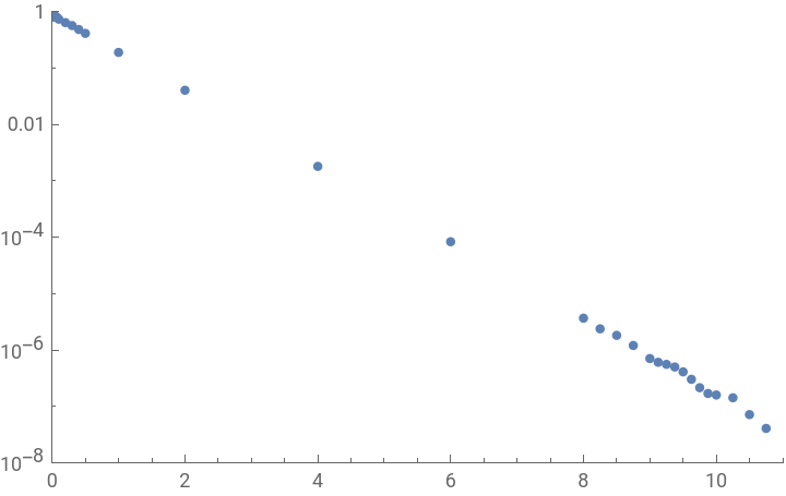
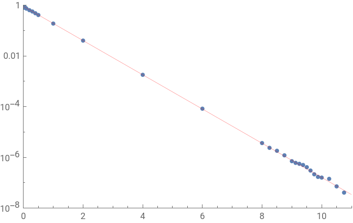
Fit the data to a decaying exponential to get the decay lifetime
In[]:=
fitData=Select[ρPlot,#[[1]]>1.5&&#[[1]]<8.5&];func=aExp[-x/τ];fitPars=FindFit[fitData,func,{a,τ},x]
Out[]=
{a0.907508,τ0.643116}
The value of τ should agree with Winter’s value 0.644 (middle, left column, page 1505)
In[]:=
fitTrue=func/.fitPars;Show[ListLogPlot[ρPlot,PlotRange{{0,11},{10^(-8),1}}],LogPlot[fitTrue,{x,0,11},PlotStyle{Thin,Red}]]
Out[]=
Use the fitted lifetime to scale the results in the small and large time region
In[]:=
ρPlotScaled=Transpose[{Ts,(Exp[Ts/τ]/.fitPars)Re[ρ]}];
In[]:=
ListPlot[ρPlotScaled,JoinedTrue,MeshAll,PlotRangeAutomatic]
Out[]=
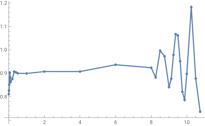
For T>8, there are oscillations with amplitude approaching 20% on top of the exponential decay.
In[]:=
ListPlot[ρPlotScaled,JoinedTrue,MeshAll,PlotRange{{0,1.1},{0.8,0.92}}]
Out[]=
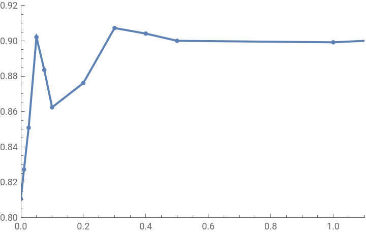
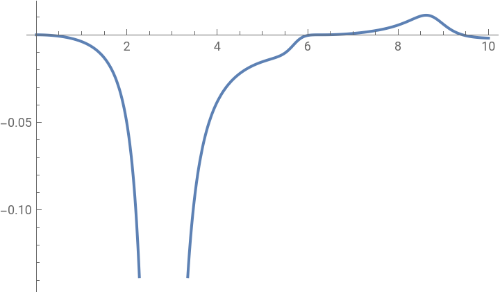
For T<0.5, there are also oscillations, but it is disturbing that the normalization doesn’t come out to unity at T=0. It’s worth doing some investigation of the integrand.
In[]:=
Plot[Integrate[intg/.vals/.f0/.T0,{l,-1,0}],{q,0,10}]
Out[]=