I am so very glad to announce the publication of a new ebook, “Signals, Systems and Signal Processing: A Computational Approach”, by Mariusz Jankowski. The topics discussed in this text are a mainstay of almost every electrical, computer, and biomedical engineering program in the United States and the world. In the US, they are typically taught in the second or third year of a four-year undergraduate program and provide a crucial gateway to more advanced engineering topics, such as control, communications, digital signal processing, image processing, machine learning, and more. They lie at the core of many applications: audio processing, speech recognition, computer vision, financial and genomic data analysis, sonar and radar and AI-enabled systems. CITATION (original book): Mariusz Jankowski (2024), Signals, Systems, and Signal Processing: A Computational Approach, Wolfram Media. ISBN-13: 978-1-57955-093-6 (digital online). https://wolfram-media.com/products/signals-systems-and-signal-processing
The book together with the accompanying Wolfram U course Signal, Systems and Signal Processing provide a comprehensive introduction to fundamental concepts in the mathematical representation, analysis and design of continuous-time and discrete-time linear time-invariant systems and the signals that appear at the inputs and outputs of such systems. The primary goal of the book and the Wolfram U course is to help students in learning and mastering the many topics, concepts and method typical of an undergraduate engineering course on signals and systems. To this end the book contains over one hundred examples and over two hundred fully solved exercises that show how to overcome some of the learning barriers by taking advantage of the computational powers of the Wolfram Language. For the more traditional learners, most examples and exercises include detailed step-by-step derivations of the solutions. You can download the ebook for free at the Wolfram Media website: wolfram-media.com/products/signals-systems-and-signal-processing.
Below are selected interactive demonstrations, chapter examples, featured applications, and exercises from the book and its accompanying solutions manual.
Demonstrations
Demonstrations
Continuous-time convolution.
DynamicModule



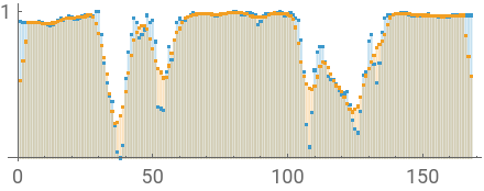
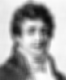
Data smoothing and image blurring using a moving-average filter of length .
N
In[]:=
Manipulate
Out[]=



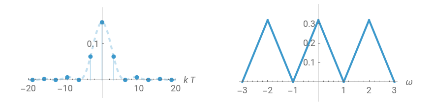
The Fourier transform (magnitude spectrum) of a sampled signal.
In[]:=
Manipulate
Out[]=
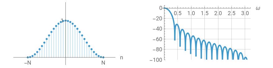
Five common window sequences and their magnitude spectra:
In[]:=
DynamicModule
Out[]=
Chapter Examples
Chapter Examples
Example 19.2
Example 19.2
Determine the discrete-time Fourier transform (DTFT) of the exponential sequence
x[n]=u[n]
n
r
r<1
Solution
Solution
First, this confirms that the given sequence is absolutely summable and therefore the Fourier transform exists:
Sum[UnitStep[n],{n,-∞,∞},GenerateConditionsTrue]
n
r
Evaluation of the DTFT returns the following result:
FourierSequenceTransform[UnitStep[n],n,ω]
n
r
ω
ω
Step-by-step
Substitute the sequence into the definition
x[n]
X()=x[n]=
jω
∞
∑
n=-∞
-jωn
∞
∑
n=0
n
r
-jωn
Rewrite the summand as , with
n
α
α=r
-jω
=
∞
∑
n=0
n
(r)
-jω
Use the well-known sum formula = to arrive at the following result
∞
∑
n=0
n
α
1
1-α
=
1
1-r
-jω
|r|<1
Example 23.1
Example 23.1
Obtain the inverse Laplace transform, given the following Laplace transform specification
X(s)=
1
(s+1)(s+3)
Re(s)>-1
Solution
Solution
Substituting the given Laplace transform and the ROC into the inverse Laplace transform function gives:
InverseBilateralLaplaceTransformConditionalExpression,Re[s]>-1,s,t//Expand
1
(s+1)(s+3)
|
This shows the signal:
Plot-+UnitStep[t],
1
2
-3t
1
2
-t
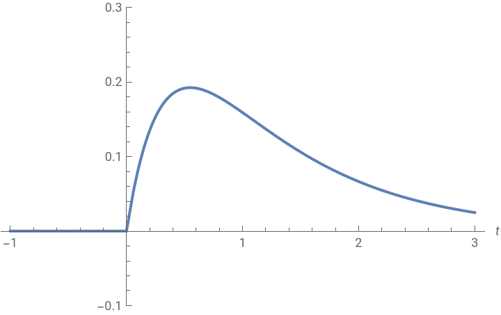
The resulting signal is causal or right sided.
Step-by-step
Partial fraction expansion of
X(s)
X(s)==+
1
(s+1)(s+3)
A
s+1
B
s+3
The values of and can be quickly obtained using the method of residues:
A
B
Limit[(s+1)X[s],s->-1]
1
2
Limit[(s+3)X[s],s->-3]
-
1
2
This gives the partial expansion as
X(s)=-
1
2
1
s+1
1
2
1
s+3
Each of the two terms can now be inverted using the transform pair
-at
ℒ
⟷
1
s+a
Re(s)>-a
For and
Re(s)>-1
a=1
1
2
1
s+1
1
2
-t
The signal takes the following form
Example 31.2
Example 31.2
In this example, the goal is to filter an audio clip of a piano key in such a way that all the low frequencies up to and including the fundamental are retained and all the higher harmonics are substantially attenuated.
Here is a clip of the sound of a piano key:
This shows the magnitude spectrum of the audio signal:
Solution
Solution
Here is a close-up of the fundamental and its first harmonic:
The desired FIR filter needs to meet the following criteria:
This returns an estimate of the length of the FIR filter:
This evaluates the normalized DTFT of the filter fir:
This plots the magnitude spectrum of the FIR filter:
This compares the magnitude spectra of the two audio clips:
Applications
Applications
The Gain Function
The Gain Function
A common laboratory experiment encountered in an introductory circuits course is to obtain the ratio of the amplitudes of the input and output sinusoidal signals over a range of frequencies. Typically, a simple RC circuit, a function generator, and an oscilloscope are used to conduct the experiment. These measurements give an estimate of the so-called gain function, a function of frequency that captures how a circuit will attenuate (or amplify) a signal over its operating range.
This compares the input to the output at each of the three frequencies
Here is a list of measurements obtained from the actual physical circuit, shown in the format {frequency in KHz, gain value}:
This plots the measurements and compares them to the circuit’s ideal gain function:
The Sound of a Piano Key
The Sound of a Piano Key
Here is a linear combination of the fundamental and its three lowest-order harmonics:
Here is what this synthesized piano key sounds like:
Exercises
Exercises
Exercise 15.2
Exercise 15.2
Obtain the continuous-time Fourier transform of the following signal.
Exercise 17.6
Exercise 17.6
Given an ideal filter with frequency response
Exercise 29.3
Exercise 29.3
CITE THIS NOTEBOOK
CITE THIS NOTEBOOK
Signals, systems, and signal processing: a computational approach
by Mariusz Jankowski
Wolfram Community, STAFF PICKS, October 18, 2024
https://community.wolfram.com/groups/-/m/t/3299985
by Mariusz Jankowski
Wolfram Community, STAFF PICKS, October 18, 2024
https://community.wolfram.com/groups/-/m/t/3299985