String hashing is a commonly used algorithm in programming that is used to quickly compare the contents of strings by assigning a string to an integer value as the comparison of integers is faster than comparing strings. To handle collisions when two strings receive the same integer value, we can use a probing algorithm to find empty spaces in the hash table. In this project, I implemented multiple hashing functions, as well as two probing algorithms in different dimensions. I then tested the different algorithms on varying datasets and used the data to analyze and compare the functions and algorithms themselves. I also used hash probing on a grid in order to generate fixed minesweeper grids based off of lists of words as an extension.
Introduction and Background
Introduction and Background
Definition of String Hashing
Definition of String Hashing
Say that we want to compare two strings efficiently. If we simply checked for equality using builtin equality checking functions, we would end up with a time complexity of ) where andarethe lengths of the two strings. However, we are able to do better; we can use an algorithm called string hashing, which is where a list of strings are mapped to integers, so that we can compare the two Strings in O(1).
However, to do this, we need a Hash Function, which is responsible for creating the map between the strings and the integer hash. For example, the builtin Wolfram data type association can be a Hash Function:
O(min(,)
N
1
N
2
N
1
N
2
However, to do this, we need a Hash Function, which is responsible for creating the map between the strings and the integer hash. For example, the builtin Wolfram data type association can be a Hash Function:
In[]:=
hashFunction=<|"cat"->1,"dog"->2,"bird"->3|>;
This function could take in “cat” and return the hash of 1 and so on.
In this computational essay, in regards to string hashing, we will:
1. talk about multiple hashing algorithms, their respective performances, and how they handle collisions
2. analyze distributions and shapes of “clusters,”
3. apply hashing in a rather unexpected manner.
In this computational essay, in regards to string hashing, we will:
1. talk about multiple hashing algorithms, their respective performances, and how they handle collisions
2. analyze distributions and shapes of “clusters,”
3. apply hashing in a rather unexpected manner.
Defining Collisions
Defining Collisions
With more complex hashing functions, there arises a possible issue: the issue of collisions. One example of a collision is shown below; the very poor hashing function would evaluate the same value for both strings, which is definitely not good for the purpose of comparison.
A hash function that outputs the same result for two distinct words:
In[]:=
hashFunction[word_String]:=StringLength[word];hashFunction["cats"]hashFunction["dogs"]
Out[]=
4
Out[]=
4
Obviously, if we tried to compare these two strings, we would get results that are less than optimal - we would get that these two strings are the same under the hash, when they are in fact different. This can be a major problem, especially in real word contexts of hashing application, where hashing is used in cybersecurity and fraud detection, such as being used to verify the integrity of files to make sure they are not tampered with.
Handling Collisions
Handling Collisions
To handle collisions, we will introduce an algorithm known as probing. Probing is the process of, given two words that hash to the same value, reassign the value of one of them in order to avoid collisions. For example, one of the most simple probing algorithms is linear probing, where, when two values collide, we search forward through the hash table until we reach an open memory location. The algorithm for string hashing can be seen in the multiway systems for hash tables of length 2 and 3 below:
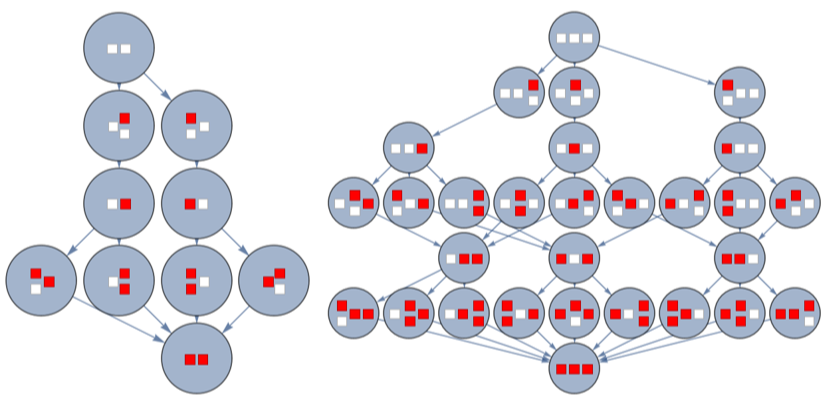
In the multiway system above, layers alternate between being “states” and “events” where all possible results of the next hash are described by events, before each of these events themselves are then converted to the next state. A column consisting of a red square and another square under it represents an event where we try to place a string in that position, and with the event nodes, we are fairly easily able to trace how the probing algorithm handles collisions.
Functions: Hashing and Probing
Functions: Hashing and Probing
Hashing Algorithms
Hashing Algorithms
Generally, I will be using three different hashing functions during the course of the project. I will compare and contrast these three algorithms in terms of collision efficiency, clustering behavior, and will also perform additional deep dives and individual analysis on them.
Random Choice
Random Choice
The random choice algorithm is the most basic possible hashing function that will generally be used as a benchmark and a comparison, as well as a tool to test out large amounts of computation due to its efficiency. The function randomChoiceHash takes in two arguments, tableLength describing the length of the hash table and word describing the word, and works by selecting an arbitrary integer to assign to any word, given the size of the hash table and the word itself.
A function that chooses a random position to put the string in the hash table:
In[]:=
randomChoiceHash[tableLength_Integer,word_String]:=RandomInteger[{1,tableLength}]
One strength of this function is the absence of needing a proper and varied list of random strings to generate results, as well as being able to run in constant time, which allows it to run quickly which is helpful for basic analysis.
Builtin Function
Builtin Function
The second function that I will use is a modification upon the builtin wolfram hash function. This function takes in the same two arguments as above, but this time uses the builtin Hash function with modulus to make sure the hash stays on the table and modulus to take into account wolfram language’s system of one-indexing.
A hashing function that slightly modifies wolfram’s builtin hashing function:
In[]:=
builtinHash[tableLength_Integer,word_String]:=Mod[Hash[word]-1,tableLength]+1
I will be comparing wolfram’s builtin hashing function with other functions and testing how well it holds up.
Polynomial Rolling Hash
Polynomial Rolling Hash
The final function that I will use will be the polynomial rolling hash, a commonly used algorithm in competitive programming. This function takes in the same two arguments as above, but changes every character to a number between 0-25 and then treats it as an integer in base 31, before converting that to base 10 and taking modulus.
A function that implements the polynomial rolling hash:
In[]:=
polynomialRollingHash[tableLength_Integer,word_String]:=(Mod[Sum[(ToCharacterCode[Characters[ToLowerCase[word]][[i]]]-97)*31^i,{i,StringLength[word]}]-1,tableLength]+1)[[1]]
For this hashing function specifically, I will be doing an analysis on how the choice of the base impacts the quantity of collisions. However, for most portions of this computational essay, I will be considering the base to be 31 due to it being a very commonly used number for being a prime number close to 26, the amount of letters in the alphabet.
Probing Algorithms: Linear Probing
Probing Algorithms: Linear Probing
The linear probing algorithm, as described above, is the most simple probing algorithm and effectively chooses the next empty position on the hashing table, in order to place the word in the case of collisions. My code takes in three arguments, the integer argument htLength describing the length of the hashing table, the list argument elements describing the list of words, and the argument hashFunc describing which function we will be using for the probing . It uses the FirstPosition function in order to find the first occurrence of an empty position following the position given by the hashing algorithm, as well as using a variable to track the amount of collisions and an association to track the hashes, before returning the final filled hash table, the amount of collisions that occurred during the hash, and the association describing the hashes
The linearProbing function which performs linear probing:
In[]:=
linearProbing[htLength_Integer,elements_List,hashFunc_]:=Module[{hashTable=Table[False,htLength],collisionCount=0,hashes=<||>},Table[Module[{currentPos=hashFunc[htLength,elements[[i]]]},firstPos=FirstPosition[Join[hashTable[[currentPos;;]],hashTable[[;;currentPos-1]]],False][[1]];collisionCount+=firstPos-1;AppendTo[hashes,Mod[(currentPos+firstPos-2),htLength]+1->elements[[i]]];hashTable[[Mod[(currentPos+firstPos-2),htLength]+1]]=True],{i,1,Length[elements]}];{hashTable,collisionCount,hashes}]
A hash table that shows which spaces are filled:
In[]:=
result=linearProbing[50,Table[RandomWord[],25],builtinHash];result[[1]]
Out[]=
{False,True,False,False,True,False,False,False,False,False,False,False,True,True,True,True,True,True,True,False,False,True,False,True,True,True,False,False,True,False,False,False,True,True,True,True,True,False,False,False,False,False,True,True,True,False,False,True,True,True}
The amount of collisions that occurred:
In[]:=
result[[2]]
Out[]=
15
An association describing each string:
In[]:=
result[[3]]
Out[]=
2disassociation,26perturbing,43homeward,13crosspiece,37quilting,15unsung,34cubicle,33inadvertence,16truancy,14friction,35tabulation,24technophobia,17bonk,22heterozygous,5learnedly,48muleteer,49anatomic,50daguerreotype,18naughty,44pliability,25bedimmed,36disorienting,19overwinter,45lengthen,29rhinestone
Probing Algorithms: Probing on a Grid
Probing Algorithms: Probing on a Grid
When we talk about probing on a grid, we generally refer to probing on a graph with edges connecting cells that would be adjacent in the grid. This is because it is far easier to search through a graph using builtin functions.
Generating a Torus Graph
Generating a Torus Graph
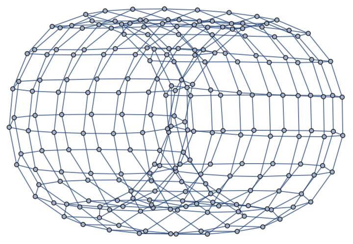
To implement grid probing, we first need a method to generate a torus graph, or a graph of a grid which can loop around, accounting for the modulus of probing algorithms. This function takes in an integer argument size which describes the side length of the square grid the torus graph is representing, and returns the torus graph by creating an edge if it detects that these two nodes would be adjacent in the table.
A function that generates a torus graph:
In[]:=
generateGridGraph[size_Integer]:=Graph[DeleteDuplicates[Flatten[Table[{If[Mod[i,size]==0,ii-size+1,ii+1],If[i>size*(size-1),i(i-size*(size-1)),i(i+size)]},{i,size^2}]]]]
A torus graph of side length 15:
In[]:=
generateGridGraph[15]
Out[]=
Implementation of Grid Probing
Implementation of Grid Probing
We will also implement probing on a grid instead of a linear table, and compare the two methods. The algorithm for probing on a grid is to, in the case of collisions, look for free spaces by checking cells based on distance from the initial cell until we find one that is unfilled. I implemented the code using the builtin function BFS which can be used to generate a list of nodes based on distance from a certain node. After this, I used a similar method to the linear probing algorithm to find the closest element. This function takes in the same arguments as the function above.
The gridProbing function which performs grid probing:
In[]:=
gridProbing[htLength_Integer,elements_List,hashFunc_]:=Module[{hashTable=Table[False,htLength],collisionCount=0,graph=generateGridGraph[Sqrt[htLength]],hashes=<||>},Table[Module[{currentPos=hashFunc[htLength,elements[[i]]],order={},order2={}},BreadthFirstScan[graph,currentPos,{"PrevisitVertex"->(AppendTo[order,hashTable[[#]]]&)}];BreadthFirstScan[graph,currentPos,{"PrevisitVertex"->(AppendTo[order2,#]&)}];collisionCount+=(Position[order,False][[1]][[1]]-1);hashTable[[order2[[Position[order,False][[1]][[1]]]]]]=True;AppendTo[hashes,order2[[Position[order,False][[1]][[1]]]]->elements[[i]]];graph=HighlightGraph[graph,{order2[[Position[order,False][[1]][[1]]]]}]],{i,1,Length[elements]}];{hashTable,collisionCount,graph,GraphicsGrid[Table[Table[If[hashTable[[Sqrt[htLength]*(i-1)+j]],Graphics[{Red,Rectangle[]}],Graphics[{White,Rectangle[]}]],{j,Sqrt[htLength]}],{i,Sqrt[htLength]}],FrameAll],hashes}]
This code outputs a list containing the hash table, the quantity of collisions, an image of the graph with filled nodes highlighted, a grid which also shows which elements are highlighted (an accurate way to visualize the end result) and an association describing the hashes.
The hash table describing which positions are filled:
The amount of collisions that occurred in the process of the probing:
The final state of the graph with filled nodes highlighted:
The filled final state of the grid:
The association of the strings and hashes:
In particular, one might notice that the clusters in the grid from above seems to look very random and doesn’t cluster in a way that one might expect. This detail will be explored later.
Analysis
Analysis
Quantity of Collisions
Quantity of Collisions
In this section, we analyze the quantity of collisions that occur on different data sets as well as differing hashing and probing algorithms. The goal of this section is to have a better understanding on what could be a factor that influences the amount of collisions, which directly impacts the time that the algorithm can take to run.
Linear Collisions
Linear Collisions
First, I will analyze the amount of collisions on a linear hash table using linear probing. The first step for this would be to initialize the data sets and collision data, which is a table of results from running linear probing with each hashing method 100 times in a hashing table of size 100 with 50 elements.
Code that generates data for Linear Collisions:
A bar chart with the mean, minimum, and maximum amount of collisions in these runs:
There are a few interesting aspects of this bar chart. The first, and perhaps most unexpected aspect, is that the random choice function actually outperformed both the builtin and the polynomial rolling hash in terms of both average collision count and deviation. Another aspect that I found surprising was the fact that the averages for all of the functions were actually relatively similar; implying that both the builtin and the polynomial rolling functions perform very similarly to a completely randomly chosen integer.
Grid Collisions
Grid Collisions
I will also analyze the amount of collisions on a grid hash table using graph probing. Once again, similarly, I will initialize the data sets and collision data, running the same table with 100 runs of each function on a 100 element hash table with 50 words to fill in .
Code that generates data for grid probing:
Bar chart with the mean, minimum, and maximum amount of collisions for the dataset:
There are also a few things to note here. One of the takeaways from this data set is that the average amount of collisions from the Polynomial rolling hash is noticeably lower than the other two functions, contradicting the result on the linear hash table. Another thing that I noticed was that the maximum amount of collisions was lower for every function, showing less deviation between runs.
Comparing Between Different Functions
Comparing Between Different Functions
Another comparison I did was how the amount of collisions rises as the hash table fills up between all three functions, and contrasted the functions themselves by using a line plot. However, the comparison actually gave surprising results. In the block of code below, I create a line plot which shows three different line plots that describe an average in the amount of collisions based on how filled the hash table is.
Line plot that describes the average amount of collisions as the table fills:
Upon inspection, one can make two observations:
(1) The three curves match nearly perfectly, showing that the three functions actually perform very similarly under the linear probing algorithm.
(2) We can also view the graph as a polynomial graph, as the expected amount of collisions is a function based on squares of the lengths of each contiguous cluster.
Cluster Analysis
Cluster Analysis
We have danced around the idea of clusters for a while but have never seriously gone to analyzing them. First, we must constitute what describes a cluster.
In linear hashing table, a cluster is defined as a contiguous sequence of cells that are occupied, while in a grid, a cluster is defined as a group of cells that are all adjacent to at least one other cell in that group (e.g. sharing a side in a cardinal direction).
In linear hashing table, a cluster is defined as a contiguous sequence of cells that are occupied, while in a grid, a cluster is defined as a group of cells that are all adjacent to at least one other cell in that group (e.g. sharing a side in a cardinal direction).
Linear Clusters
Linear Clusters
First, we analyze how linear clustering tends to behave in one dimensional hash tables.
However, we first need a function that can find clusters given a filled hash table. Here, I have created a function that is able to find the amount of clusters in a one dimensional hashing table given which cells are filled, given the hashing table as well as the total amount of filled cells. This function uses the builtin table function in order to iterate through the hashing table and keeps a running counter of the length of the current cluster.
However, we first need a function that can find clusters given a filled hash table. Here, I have created a function that is able to find the amount of clusters in a one dimensional hashing table given which cells are filled, given the hashing table as well as the total amount of filled cells. This function uses the builtin table function in order to iterate through the hashing table and keeps a running counter of the length of the current cluster.
A function that finds all clusters in a linear function:
The function itself returns a list of small, medium and large clusters, where a large cluster is considered a cluster that contains more than one fifth of the total elements, a medium cluster is considered one that contains between one tenth and one fifth of the total elements, and a small cluster is considered to be any other cluster. Using this function as well as the previously obtained data, we can compile and define some new datasets describing the three different hashing functions.
Generating the cluster data for three different hashing functions:
Bar chart of the data:
This bar chart has a few interesting things to observe. First off, the amount of collisions for all three hashing functions seem to be very similar and vary very minimally, which is relatively similar to the former observations that we have made. Another notable observation is that on average, nearly 90% of clusters are small. This shows that in linear hashing, a significant amount of clusters are very small; it is very rare to end up with a massive cluster, something that evidently does not become the case for grid probing, which will be analyzed later.
Cluster Distribution Comparison
Cluster Distribution Comparison
Afterwards, I did an analysis how the amount of clusters change based off of how filled in the hash table is by finding the average amount of clusters for each size of the list of elements, and compared and contrasted the distribution of grid probing and linear probing to see the difference between the two algorithms. For the linear probing algorithm, I created a bar chart that runs each element count 30 times on a hash table of size 100, using linear probing as well as a hashing function to generate the final state of the hash table and the previously mentioned clusterFind function.
A bar chart that shows the amount of clusters as the hash table fills up:
Evidently, the quantity of clusters peaks when around half of the grid is filled before dropping off. This makes sense because the larger the amount of elements, the more likely they are to form a massive cluster instead of being small clusters, until when the grid is fully filled in which the elements must all form one connected cluster. We can note that the amount of clusters peaks at around 20, but when we run the same algorithm for a grid, we get very different results.
However, to perform this algorithm, we first need to define a function that can compute the “clusters” in the grid. The clusterGridFind function takes in a hash table as well as a graph, creating a new graph consisting of only highlighted nodes by creating all edges between filled nodes as well as initializing the filled nodes themselves, before returning the connected components in that array.
However, to perform this algorithm, we first need to define a function that can compute the “clusters” in the grid. The clusterGridFind function takes in a hash table as well as a graph, creating a new graph consisting of only highlighted nodes by creating all edges between filled nodes as well as initializing the filled nodes themselves, before returning the connected components in that array.
A function that outputs connected components in a grid:
A bar chart that keeps track of the amount of clusters in probing on a grid:
Although this shares some properties with the first curve, namely the idea that the amount of clusters starts low, reaches a peak, and then drops off as the amount of clusters increases, there are many notable differences, one being the overall shape of the curve, taking the appearance of a right skewed distribution; when the amount of elements in the array reaches around half, we only get an average of 2 to 3 clusters, and we peak at around 30 elements in the array. Another difference is the maximum amount of clusters; while the linear algorithm peaked around 12 clusters as opposed to the 20 that the linear algorithm peaked around. This implies that on average in a grid, we have larger clusters, but less of them.
Cluster Density
Cluster Density
Another topic that will be analyzed is the “blobbiness” of a cluster in a grid, which was briefly mentioned above. In general, when someone thinks about a blob, they think of something like this:
However, as you may have guessed from an example grid from some above code, most blobs don’t end up being condensed and instead consist of thin connected segments pointing outwards. In fact, that above output took a pretty considerable amount of runs to generate such a nice blob. Most clusters end up looking like this, rather than the above:
Both clusters contain all filled squares, but there is a significant difference in overall shape: the one on top has all elements clustered together, while the one on the bottom consists of cells that are primarily only adjacent to one other cell in the cluster, increasing the span of the cluster. We will thus analyze the “blobbiness” of clusters; e.g. their overall shapes to find out how clusters interact under the grid hashing algorithm.
An idea to think about is how one quantifies how “blobby” a cluster is. For the purpose of this essay, I will treat the blobbiness of a cluster as the “density,” or the fraction of the amount of space it takes up inside of its bounding box. For the purpose of this analysis, we define a function that takes in a list, “components”, which is the connected components of a graph . Based on this list, the function finds the length and width of the bounding box, before returning a list of the densities.
An idea to think about is how one quantifies how “blobby” a cluster is. For the purpose of this essay, I will treat the blobbiness of a cluster as the “density,” or the fraction of the amount of space it takes up inside of its bounding box. For the purpose of this analysis, we define a function that takes in a list, “components”, which is the connected components of a graph . Based on this list, the function finds the length and width of the bounding box, before returning a list of the densities.
A function that returns a list of the densities of each component:
A bar chart which compiles the average densities for each size of cluster:
Once again, there are a few interesting takeaways from this graph. for example, one thing that we can note is the shape, where it appears that clusters of smaller size start off being very dense before quickly dropping to a low density before returning to a high density. This is due to small clusters not having enough configurations that have low densities, while large clusters filling up a large enough portion of the grid to allow the bounding box of the grid to be fixed. Another interesting observation is that at the end of the graph, the density appears to rise in a linear fashion; this is caused by clusters having large sizes to have a bounding box that spans the whole grid, and the density merely being decided by the size of the cluster.
Individual Function Analysis
Individual Function Analysis
Polynomial Rolling Hash: How Modulo Impacts Results
Polynomial Rolling Hash: How Modulo Impacts Results
One final analysis came from specifically the polynomial rolling hash function, for which the behavior can change depending on which base we use as the prime. In general, all of our analysis thus far has come from using 31. However, what if we decided to change the base and analyze the amount of collisions stemming from that? Our first step in this is to add an additional parameter to both our polynomial rolling hash function and our our linear probing function.
A modified polynomial rolling hash function that allows for base change:
A function that finds the cycle of an exponent of a certain prime:
A graph of the average collision count and the cycle length for primes:
The above graph is very interesting in the sense that we can see the impact of the modulus cycle length to the average amount of collisions (where average collision count is in blue and modulo cycle length is in orange). We can see that in the case of all the major spikes have short cycle lengths, which is relatively easy to explain due to the fact that having a short cycle length mod 100 makes many letters equivalent in the hashing algorithm. For example, 199 did poorly because 199 has a cycle length of 2, and as such, every second letter is equivalent under the hashing operation.
However, there are also many interesting observations that appear from this graph: for example, primes like 101 and 401 have cycle lengths of 1, so why do these perform decently? And what makes a prime perform significantly well, where cycle length seems to have relatively minimal correlation? Unfortunately, I did not have enough time to do a detailed explanations of these facts, but I would like to try them in the future as a future path that could be taken.
However, there are also many interesting observations that appear from this graph: for example, primes like 101 and 401 have cycle lengths of 1, so why do these perform decently? And what makes a prime perform significantly well, where cycle length seems to have relatively minimal correlation? Unfortunately, I did not have enough time to do a detailed explanations of these facts, but I would like to try them in the future as a future path that could be taken.
Fun Applications
Fun Applications
Minesweeper
Minesweeper
After the successful development of a successful hash probing algorithm on a grid, we can now use the grid for a multitude of purposes, such as generating some interesting applications. One of which is minesweeper, from which we can take in a list of words, hash them into a grid, and then generate a minesweeper board based off of the configuration, using a function that creates a minesweeper grid, places bombs at every element that is occupied by a word, and fills in the remaining spaces with the number that describes the amount of bombs neighboring it.
A function that generates a minesweeper grid off of a list of words:
We can now initialize some variables for the game:
Code that generates the starting state of the grid:
The logic and display of the game:
When put together, we get a working game that generates a unique minesweeper board for lists of strings!
Unfortunately, due to the dynamics not working on cloud, the game is not playable. However, here are some screenshots of the game being played for the sentence, “Wolfram summer research program twenty two thousand twenty four” with the start of the game, a partially completed board, and a game over.
Unfortunately, due to the dynamics not working on cloud, the game is not playable. However, here are some screenshots of the game being played for the sentence, “Wolfram summer research program twenty two thousand twenty four” with the start of the game, a partially completed board, and a game over.
Conclusion
Conclusion
Concluding Thoughts and Future Directions
Concluding Thoughts and Future Directions
It is fairly surprising that such a simple idea, the idea of hashing, a basic algorithm in programming, could end up with so many different directions to explore. There are multiple different comparisons that one is able to make, whether it be between hashing functions, between dimensions, or even specific parameters of some of these functions. In this project, I successfully created multiple hashing and probing functions, tested them on a variety of datasets, and compared and contrasted the results. I also used the functions in a pretty interesting way as a way to generate minesweeper boards.
There are many interesting ideas that I could implement, one of which is a better analysis on modulus because I am curious to find a deeper explanation on why some modulo work better than others. I would also like to find a way to mathematically predict the amount of collisions by generalizing and finding an equation that describes the graph to be able to more clearly analyze the behavior of certain graphs. I would also try to expand the computations that I have done to three dimensions and compare how the functions interact in higher dimensions, and finding a generalization. Another extension is to find a function that can optimize the amount of collisions and lower computational time.
There are many interesting ideas that I could implement, one of which is a better analysis on modulus because I am curious to find a deeper explanation on why some modulo work better than others. I would also like to find a way to mathematically predict the amount of collisions by generalizing and finding an equation that describes the graph to be able to more clearly analyze the behavior of certain graphs. I would also try to expand the computations that I have done to three dimensions and compare how the functions interact in higher dimensions, and finding a generalization. Another extension is to find a function that can optimize the amount of collisions and lower computational time.
Acknowledgements
Acknowledgements
First off, I would like to thank my mentor, Drake Hayes, for helping me with code and providing support during the entirety of this project. I would also like to thank Stephen Wolfram for advice and help with extending my project, as well as the program directors Rory, Megan, and Eryn for hosting this amazing summer program, as well as everyone else at camp for making this experience truly one of a kind.
Citations
Citations
1
.String Hashing - Algorithms for Competitive Programming. (n.d.). Cp-Algorithms.com. https://cp-algorithms.com/string/string-hashing.html
2
.String hashing using Polynomial rolling hash function. (2020, July 20). GeeksforGeeks. https://www.geeksforgeeks.org/string-hashing-using-polynomial-rolling-hash-function/
3
.Wikipedia Contributors. (2019, November 20). Linear probing. Wikipedia; Wikimedia Foundation. https://en.wikipedia.org/wiki/Linear_probing
4
.learn hash table the hard way -- part 1: probe distributions - Carpe diem (Felix’s blog). (n.d.). Www.idryman.org. Retrieved July 10, 2024, from https://www.idryman.org/blog/2017/07/04/learn-hash-table-the-hard-way/
CITE THIS NOTEBOOK
CITE THIS NOTEBOOK
Study of hash probing on a graph
by David Wang
Wolfram Community, STAFF PICKS, July 12, 2024
https://community.wolfram.com/groups/-/m/t/3215183
by David Wang
Wolfram Community, STAFF PICKS, July 12, 2024
https://community.wolfram.com/groups/-/m/t/3215183