Wolfram Cloud Document

This animation uses the modular flow to produce a periodic family of quasi-periodic functions. Since the family is periodic, we get a looping animation by visualizing with domain coloring. This is also explained in my paper "Looping animations using the modular flow and elliptic functions."

ABSTRACT (original article): This paper describes an approach to generating looping animations using the modular flow and elliptic functions. The modular flow is a flow on lattices with many periodic orbits, and elliptic functions are meromorphic, doubly-periodic functions which can be visualized using domain coloring. CITATION (original article): Clayton Shonkwiler (2026), Looping Animations Using the Modular Flow and Elliptic Functions, Proceedings of Bridges 2026: Mathematics and the Arts, 533--536. http://archive.bridgesmathart.org/2026/bridges2026-533.html

The Modular Flow

See the links which include the phrase “modular flow” in the previous paragraph for more, but for the modular flow the idea is that we will let



act on

2



by

t·(x,y):=(

t



x,

-t



y)

. As an action on the plane, this is very far from being periodic, but we can also think of the induced action on lattices

Λ={m

u

1

+n

u

2

:m,n∈}

, and if we choose

u

1

and

u

2

carefully, the resulting orbit will be periodic; that is, there will exist

t

0

≠0

so that

t

0

·Λ=Λ

.

To figure out some

Λ

for which this works, let’s turn this into a matrix problem. Let

U

be the

22

matrix with columns

u

1

and

u

2

. Then the lattice

t·Λ

will be generated by the columns of

t 	0
0	-t 

U

. On the other hand, if

B=

a	b
c	d



is an integer matrix, then the columns of

UB

will be integer linear combinations of

u

1

and

u

2

; that is, elements of

Λ

. So we might hope that the columns of

t 0 	0
0	- t 0 

U

will be the columns of

UB

. Moreover,

det

t 	0
0	-t 

=1

, so the action on

2



is area-preserving, and we can only hope for this to work if

detB=1

as well.

In other words, if we’re looking for a periodic lattice, we can try to solve the equation

UB=

t 0 	0
0	- t 0 

U

for

U

and

t

0

, where

B

is our favorite

22

matrix with determinant 1.

Taking the transpose of both sides, we see that the rows of

U

must be eigenvectors of

T

B

with corresponding eigenvalues

±

t

0



. So for example when

B=

2	1
1	1



we have:

In[]:=

Eigensystem[{{2,1},{1,1}}]

Out[]=



1

2

(3+

5

),

1

2

(3-

5

),

1

2

(1+

5

),1,

1

2

(1-

5

),1

That is,

u

1

=

ϕ

1



,

u

2

=

-1/ϕ

1



, and

t

0

=ln(1+ϕ)

, where

ϕ=

1+

5

2

is the golden ratio. In fact, I could just as well scale

u

2

by

-ϕ

to get the more pleasing

U=

ϕ	1
1	-ϕ

. Let’s visualize this and see that it really is periodic:

In[]:=

DynamicModule[{M,pts,U={{GoldenRatio,1},{-1,GoldenRatio}}},pts=Flatten[Table[{x,y},{x,-15,15},{y,-15,15}],1];Animate[M=DiagonalMatrix[{

s

E

,

-s

E

}].U;Graphics[{Thickness[.005],PointSize[Large],Point[M.#]&/@pts},PlotRange->10],{s,0,Log[1+GoldenRatio]},SaveDefinitions->True,AnimationRunning->False]]

Out[]=

s

A Quasiperiodic Function

Now, think of the lattice

Λ

as living in



rather than in

2



. That is, we now think of

Λ={m

ω

1

+n

ω

2

:m,n∈}

where

ω

1

,

ω

2

∈

. And, for any such lattice we can think about doubly-periodic functions with periods

ω

1

and

ω

2

; that is, functions

f:

so that

f(z+

ω

1

)=f(z)=f(z+

ω

2

)

, which of course implies

f(z+m

ω

1

+n

ω

2

)=f(z)

for all

m,n∈

. If such an

f

is meromorphic then it is usually called an elliptic function.

This is the idea behind the animation Phase, where I applied this idea to the most basic elliptic function, the Weierstrass

℘

-function. Since this function depends on the lattice

Λ

, I like to write it as

℘

Λ

(z)

, though it’s more common to write

℘(p;

ω

1

,

ω

2

)

or

℘(z;

g

2

,

g

3

)

, where

g

2

,

g

3

are the Weierstrass invariants of

Λ

, and indeed this latter is how Mathematica works. In the below code, I translate back and forth between

(

ω

1

,

ω

2

)

and

(

g

2

,

g

3

)

using the built-in Mathematica function WeierstrassInvariants.

In any case, the point is that if we have a periodic family

t·Λ

of lattices, then the corresponding family

℘

t·Λ

is also periodic (and likewise for any other elliptic function), and so produces a looping animation when visualized.

Here I’m going to apply the same idea to a quasiperiodic function, namely the Weierstrass

σ

Λ

function, which is implicitly defined by

2

d

2

z

ln(

σ

Λ

)=-

℘

Λ

. This function is entire and can be used to represent all elliptic functions by way of their zeros and poles. Plus, it looks weird and interesting:

In[]:=

ComplexPlot[WeierstrassSigma[z,WeierstrassInvariants[{1,I}]],{z,10}]

Out[]=

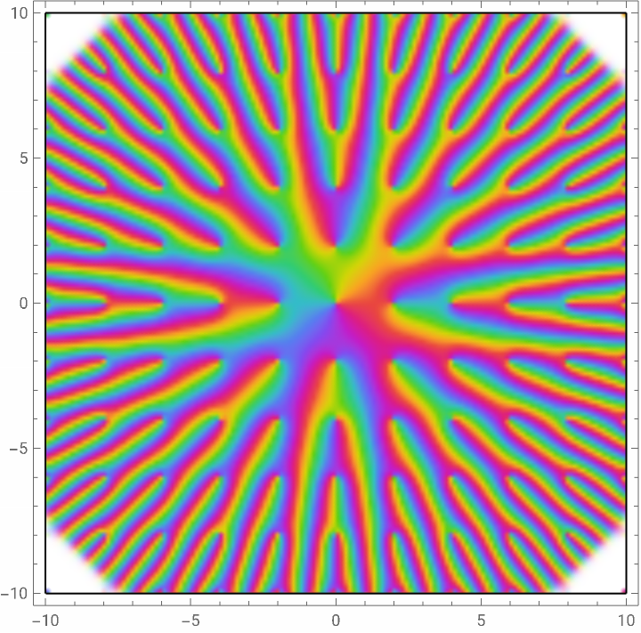
Putting it all together, we’re going to let

Λ

be the lattice generated by



ϕ

1



and



1

-ϕ



(or, in complex terms,

ϕ+

and

1-ϕ

), we’re going to let

t·Λ

be its periodic orbit under the modular flow (with period

t

0

=ln(1+ϕ)

), and we’re going to build the corresponding periodic family of quasiperiodic functions

σ

t·Λ

, which we’ll visualize and turn into a looping animation using domain coloring.

For this, I’m using the vik0 cyclic gradient from Scientific Color Maps:

In[]:=

cols={

,

};

To get the look I wanted, I rotated this palette a quarter-turn, which explains the Mod[#8 - 1/4, 1] in the code, which I can now give:

quasi=Module{g2,g3,U={{GoldenRatio,1},{1,-GoldenRatio}}},ParallelTable{g2,g3}=WeierstrassInvariants[N[Complex@@(DiagonalMatrix[{

s

E

,

-s

E

}].U.#)]&/@{{1,0},{0,1}}];ComplexPlotWeierstrassSigma[z,{g2,g3}],{z,20},ColorFunction{Blend[cols,Mod[#8-1/4,1]]&,None},

,{s,0.,Log[1+GoldenRatio]-#,#}&[Log[1+GoldenRatio]/70.];

Which we can export to a GIF:

Export[NotebookDirectory[]<>"quasi.gif",quasi,"AnimationRepetitions"->Infinity,"DisplayDurations"->1/50];

Or visualize using ListAnimate:

In[]:=

ListAnimate[sigmaframes,50]

CITE THIS NOTEBOOK

Quasi (periodic family of quasiperiodic functions)
by Clayton Shonkwiler
Wolfram Community, STAFF PICKS, June 15, 2026
https://community.wolfram.com/groups/-/m/t/3734174