S23OrderDistribution tits to DJIA from 1900 to 1950
S23OrderDistribution tits to DJIA from 1900 to 1950
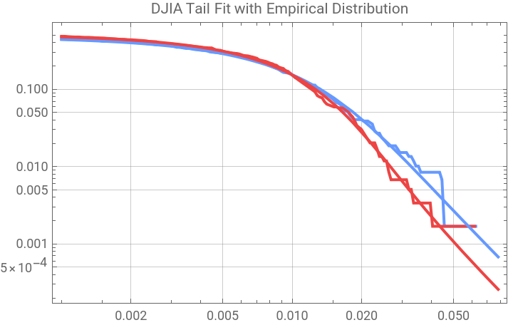
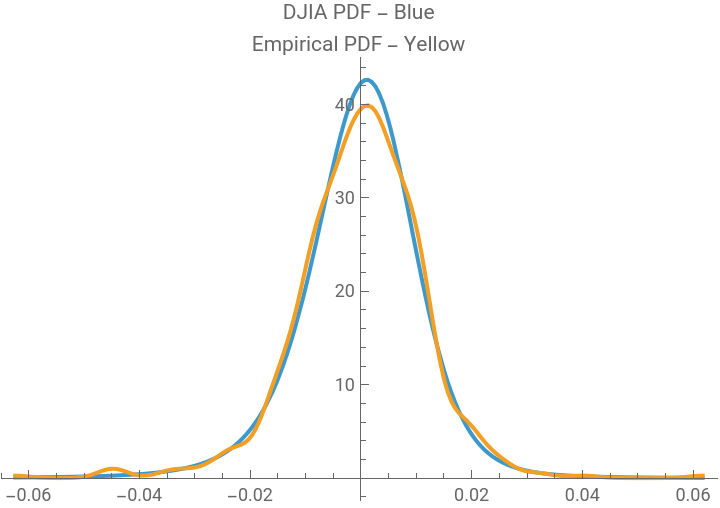
This notebook fits the Dow Jones Industrial Average in two year intervals to an S23OrderDistribution with good quality results. Apparently market log returns have a distributional shape which has not changed since all the trades were executed by hand and the best information technology was telephone and ticker tape, both of which generally failed in extreme markets. Human behavioral interactions with financial markets does not seem to be affected much by modern technology.
This is an extended data set of the Dow Jones Industrial Average obtained from https://www.measuringworth.com/datasets/DJA/. It includes Saturday trading in the early series.
In[]:=
djiaT=ImportByteArrayByteArray
Out[]=
Tabular


In[]:=
Needs["S23OrderDistribution`"]
In[]:=
tickerSymbol="DJIA";
In[]:=
Clear[S23DJIAFit];S23DJIAFit[djiaData_]:=Module[{lr,pLevel,lrQrng,lrD,parm0,skd,dt,α,β,μ,σ,s23d,HTs23d},Print[DateListPlot[djiaData,PlotRangeAll,JoinedTrue,GridLines->Automatic,PlotLabeltickerSymbol<>" Closing Price"]];(*Print[DateListLogPlot[data,PlotRangeAll,JoinedTrue,PlotLabeltickerSymbol<>" Closing Price\nLog Scale"]];*)lr=Differences[Log[djiaData[[All,2]]]];dt=Rest[djiaData[[All,1]]];pLevel=0.02;lrQrng=Quantile[lr,{pLevel,1-pLevel}];Print[DateListPlot[Tooltip@{Transpose[{dt,lr}],Select[Transpose[{dt,lr}],!lrQrng[[1]]<#[[2]]<lrQrng[[2]]&]},PlotStyle{{StandardBlue,PointSize[0.01]},{StandardRed,PointSize[0.01]}},PlotRangeAll,Joined->False,GridLines->Automatic,PlotLabeltickerSymbol<>" Daily Log Returns\np = "<>ToString[pLevel,TraditionalForm]<>" Extremes Red"]];lrD=EmpiricalDistribution[lr];s23d=EstimatedDistribution[lr,S23OrderDistribution[α,β,μ,σ]];parm0=List@@s23d;Print[tickerSymbol," Stable 2:3 Order Statistic Distribution Parameters, {α, β, μ, σ, type}:\n",parm0,"\nDistribution Fit Test"];HTs23d=DistributionFitTest[lr,s23d,"HypothesisTestData"];Print[HTs23d["TestDataTable",All],"\n"];Print[LogLogPlot[{CDF[lrD,-x],1-CDF[lrD,x],CDF[s23d,-x],1-CDF[s23d,x]},{x,0.001,Max[Abs[lr]]5/4},PlotRangeAll,PerformanceGoal"Speed",FrameTrue,GridLinesAutomatic,PlotStyle{StandardBlue,StandardRed,StandardBlue,StandardRed},PlotLabeltickerSymbol<>" Tail Fit with Empirical Distribution"]];skd=SmoothKernelDistribution[lr];Print[Plot[{PDF[s23d,x],PDF[skd,x]},{x,Min[lr],Max[lr]},PlotRangeAll,PerformanceGoal"Speed",PlotLabeltickerSymbol<>" PDF - Blue\nEmpirical PDF - Yellow"]];];
In[]:=
djiaData=Select[djiaT,DateObject[{1900,1,1}]<#Date<DateObject[{1902,1,1}]&]//Normal//Values;S23DJIAFit[djiaData]
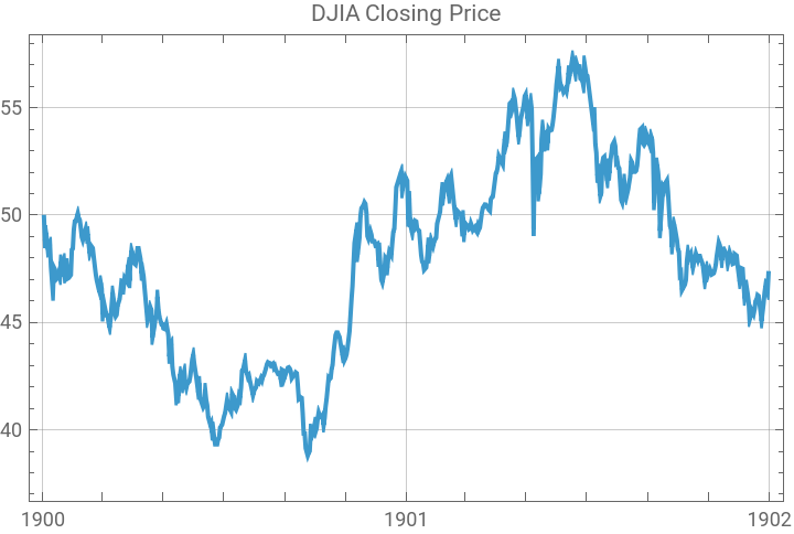
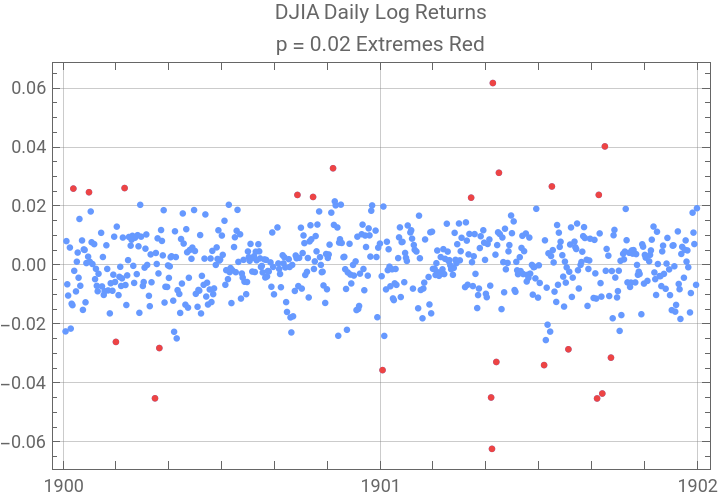

DJIA Stable 2:3 Order Statistic Distribution Parameters, {α, β, μ, σ, type}:{2.88398,-0.231366,-0.00171574,0.0101111,1}Distribution Fit Test
Statistic | P-Value | |
Anderson-Darling | 0.236162 | 0.977216 |
Cramér-von Mises | 0.0320018 | 0.969138 |
Pearson 2 χ | 33.9324 | 0.10936 |
In[]:=
djiaData=Select[djiaT,DateObject[{1902,1,1}]<#Date<DateObject[{1904,1,1}]&]//Normal//Values;S23DJIAFit[djiaData]
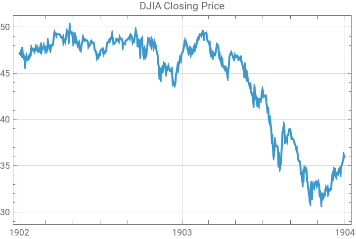
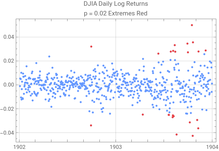
DJIA Stable 2:3 Order Statistic Distribution Parameters, {α, β, μ, σ, type}:{2.48468,-0.0638796,-0.00150395,0.00858941,1}Distribution Fit Test
Statistic | P-Value | |
Anderson-Darling | 0.203158 | 0.989528 |
Cramér-von Mises | 0.0275736 | 0.98344 |
Pearson 2 χ | 23.6252 | 0.541104 |