Guhan Thiagarajan
Quantum noise limits the reliability of quantum devices, making it essential to identify the type of noise affecting a system when the underlying model is unknown. Using the density matrix formalism, single-qubit systems are simulated under common quantum noise channels, and measurement probabilities in the computational basis are recorded. Features are extracted from these measurement-probability curves and used to train a feature-weighted multilayer perceptron (MLP) for supervised noise-channel classification. The model can differentiate among depolarizing, dephasing, amplitude-damping, bit-flip, and asymmetric depolarizing noise with approximately 89% accuracy using only measurement data. The results show that different noise channels leave clear statistical signatures in the measurement outcomes that a neural network can learn. Overall, this work exemplifies that data-driven methods can provide an effective and practical approach for diagnosing quantum noise in near-term quantum systems.
Introduction
Noise in Computing
Noise in Computing
Quantum computers are highly susceptible to noise arising from environmental interactions, control imperfections, and hardware limitations. Characterizing the underlying noise processes is a critical challenge for quantum error mitigation and device calibration, particularly when the noise model and parameters are unknown a priori. In this work, we study the problem of quantum noise channel classification in single-qubit systems using measurement statistics alone. We simulate the action of distinct quantum noise channels on a qubit prepared in a set of initial states and record the resulting probability of measuring the computational basis state ∣0⟩. These measurement probability curves encode characteristic signatures of the underlying noise process. We extract features from these curves and use them to train a feature-weighted multilayer perceptron (MLP) to classify the noise channel in a supervised learning setting. Our approach demonstrates that even limited measurement data can be leveraged to reliably distinguish between different types of quantum noise, offering a data-driven tool for noise diagnosis in near-term quantum devices.
Installation of the Quantum Framework paclet:
Installation of the Quantum Framework paclet:
In[]:=
PacletUninstall["Wolfram/QuantumFramework"]PacletInstall["https://wolfr.am/DevWQCF", ForceVersionInstall -> True]
Out[]=
PacletObject

Methods
Part 1: Simulating Quantum Noise Channels
Part 1: Simulating Quantum Noise Channels
We simulate five quantum noise channels using the Wolfram QuantumFramework, each modeled with Kraus operators based on Pauli matrices. The channels are
1
.Depolarizing Noise: Randomly applies one of the Pauli operators (X, Y, or Z) with equal probability, simulating uniform noise that pushes the qubit state toward the maximally mixed state.
2
.Dephasing Noise: Reduces coherence between |0⟩ and |1⟩ by introducing random phase shifts, causing the off-diagonal elements of the density matrix to decay.
3
.Amplitude Damping: Models energy loss to the environment (like emission), gradually pulling the qubit toward the ground state |0⟩.
4
.Bit Flip Noise: Simulates a classical bit error by flipping |0⟩ to |1⟩ and vice versa with a certain probability
5
.Asymmetric Depolarizing Noise: A variant of depolarizing noise where the X, Y, and Z errors occur with different probabilities, modeling non-uniform noise environments.
Each simulation follows these steps:
1. A qubit is initialized in the state ψ(θ), which lies on the X-Z plane of the Bloch sphere and varies from |0⟩ to |1⟩ as θ goes from 0 to π
1. A qubit is initialized in the state ψ(θ), which lies on the X-Z plane of the Bloch sphere and varies from |0⟩ to |1⟩ as θ goes from 0 to π
In[]:=
psi[θ_] := QuantumState[N[{Cos[θ/2], Sin[θ/2]}]];
The quantum state, |ψ(θ)⟩ = cos(θ/2)|0⟩ + sin(θ/2)|1⟩, is the input to each noise channel in this project. The slider below helps visualize how the state changes as θ varies from 0 to π making it easier to interpret how the noise affects different initial states.
In[]:=
Manipulate[Column[Row[{"θ = ", TraditionalForm[theta]}], Row[Style["|ψ(θ)⟩ = ", Bold], TraditionalForm[Cos[theta/2]], " |0⟩ + ", TraditionalForm[Sin[theta/2]], " |1⟩"], Row[{"State vector: ", {Cos[theta/2], Sin[theta/2]}}]], {theta, 0, Pi, Pi/6, Appearance -> "Labeled"}]
Out[]=


The noise strength parameter p is defined, which determines how likely an error occurs , and a range of θ values is defined ranging from 0 to π in steps of 0.05 radians to explore how the input state affects measurement outcomes
In[]:=
p = 0.2;thetas = Range[0, Pi, 0.05];
Each channel is defined using Kraus operators, which models how different types of noise affect the quantum state. The probZeroAfterNoise function simulates the circuit, applies the selected noise channel, and returns the probability of measuring |0⟩ in the Z-basis (which corresponds to checking the population of the |0⟩ state)
In[]:=
depChannel = QuantumChannel[{Sqrt[1 - p] IdentityMatrix[2], Sqrt[p/3] PauliMatrix[1], Sqrt[p/3] PauliMatrix[2], Sqrt[p/3] PauliMatrix[3]}];dephChannel = QuantumChannel[{Sqrt[1 - p] IdentityMatrix[2], Sqrt[p] PauliMatrix[3]}];ampDampChannel = QuantumChannel[{{{1, 0}, {0, Sqrt[1 - p]}}, {{0, Sqrt[p]}, {0, 0}}}];bitFlipChannel = QuantumChannel[{Sqrt[1 - p] IdentityMatrix[2], Sqrt[p] PauliMatrix[1]}];asymDepChannel = QuantumChannel[{Sqrt[1 - 0.3] IdentityMatrix[2], Sqrt[0.1] PauliMatrix[1], Sqrt[0.05] PauliMatrix[2], Sqrt[0.15] PauliMatrix[3]}];
In[]:=
probZeroAfterNoise[channel_, θ_] := Module[{qc, probs}, qc = QuantumCircuitOperator[{psi[θ], channel, "M"}]; probs = qc[]["ProbabilitiesList"]; probs[[1]]]
Then, we generate the probability curves for measuring 0 after different noise channels (and the ideal case) by evaluating probZeroAfterNoise over a range of angles θ. These curves allow us to directly compare how each type of noise distorts the measurement outcome relative to the ideal (noiseless) case.
In[]:=
probDepolarizing = Table[{θ, probZeroAfterNoise[depChannel, θ]}, {θ, thetas}]; probDephasing = Table[{θ, probZeroAfterNoise[dephChannel, θ]}, {θ, thetas}];probAmplitudeDamping = Table[{θ, probZeroAfterNoise[ampDampChannel, θ]}, {θ, thetas}]; probBitFlip = Table[{θ, probZeroAfterNoise[bitFlipChannel, θ]}, {θ, thetas}]; probAsymDep = Table[{θ, probZeroAfterNoise[asymDepChannel, θ]}, {θ, thetas}]; idealCurve = Table[{θ, Cos[θ/2]^2}, {θ, thetas}];
Finally, we plot the probability of measuring P|0⟩ as a function of θ for each noise channel alongside the ideal curve. Since we only measure in the Z-basis, the plotted values reflect how likely the qubit collapses to the ground state after being affected by the noise. This basis is chosen because many real quantum measurements, like in superconducting qubits, are performed in the computational basis. The differences in each curve help visualize how different noise models impact the state’s ability to stay close to |0⟩ or |1⟩ depending on the initial θ.
In[]:=
Show[ListLinePlot[{probDepolarizing, probDephasing, probAmplitudeDamping, probBitFlip, probAsymDep, idealCurve}, PlotStyle -> {Red, Blue, Green, Brown, Purple, Black}, PlotLegends -> Placed[ {"Depolarizing", "Dephasing", "Amplitude Damping", "Bit Flip", "Asymmetric Depolarizing", "Ideal"}, {Right, Top}], AxesLabel -> "θ", "P(|0⟩)", PlotRange -> {0, 1}], PlotLabel -> Style["Qubit Measurement Probabilities", 14, Black], ImageSize -> Large]
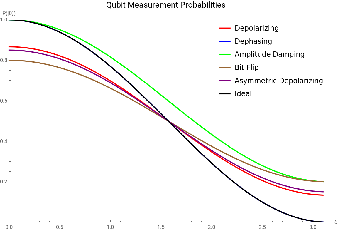
In the graph, the Dephasing curve and the Ideal curve has the same values as Dephasing noise leaves the measurement probability in the computational basis unchanged because it only affects the phase of the quantum state, not its amplitude. Since measuring in the |0⟩, |1⟩ basis ignores phase, the outcome curve is identical to the ideal case.
Part 2: Generating Noisy Curves
Part 2: Generating Noisy Curves
To train the neural network, we are generating noisy curves to simulate more realistic quantum measurements by adding small random errors on top of the noise channels. This helps to understand how actual experimental results might vary due to unpredictable fluctuations, making our analysis closer to what happens in real quantum devices.
This part follows the same steps as Part 1, but I use a density matrix (2x2) instead of a state vector because noise can turn pure states into mixed ones. The density matrix form allows quantum channels to be applied and makes it possible to track decoherence in a proper way.
This part follows the same steps as Part 1, but I use a density matrix (2x2) instead of a state vector because noise can turn pure states into mixed ones. The density matrix form allows quantum channels to be applied and makes it possible to track decoherence in a proper way.
Defining the Channels
Defining the Channels
In[]:=
ClearAll["Global`*"]sigmaX = PauliMatrix[1];sigmaY = PauliMatrix[2];sigmaZ = PauliMatrix[3];identity2 = IdentityMatrix[2];rho[θ_] := Module[{c = Cos[θ/2], s = Sin[θ/2]}, {{c^2, c s}, {c s, s^2}}];measureProbability[rho_] := Re[Tr[{{1, 0}, {0, 0}} . rho]];depolarizingChannel[rho_, p_] := (1 - p) rho + (p/3) (sigmaX . rho . sigmaX + sigmaY . rho . sigmaY + sigmaZ . rho . sigmaZ);dephasingChannel[rho_, p_] := (1 - p) rho + p (sigmaZ . rho . sigmaZ);K0[p_] := {{1, 0}, {0, Sqrt[1 - p]}};K1[p_] := {{0, Sqrt[p]}, {0, 0}};amplitudeDampingChannel[rho_, p_] := K0[p] . rho . ConjugateTranspose[K0[p]] + K1[p] . rho . ConjugateTranspose[K1[p]];bitFlipChannel[rho_, p_] := (1 - p) rho + p (sigmaX . rho . sigmaX);asymDepChannel[rho_, p_] := Module[{pX = 0.1, pY = 0.05, pZ = 0.15}, (1 - (pX + pY + pZ)) rho + pX (sigmaX . rho . sigmaX) + pY (sigmaY . rho . sigmaY) + pZ (sigmaZ . rho . sigmaZ)];
To simulate the noise within the channel more realistically, this function applies the noise to each quantum state and then adds small random fluctuations to mimic experimental imperfections. It outputs clipped probability values representing noisy measurement outcomes across different θ angles. The line
randomNoise = RandomVariate[NormalDistribution[0, 0.01], Length[thetas]];
generates random noise following a normal (Gaussian) distribution with mean 0 and standard deviation 0.01, creating a small random fluctuation for each θ value to simulate measurement errors or imperfections.
randomNoise = RandomVariate[NormalDistribution[0, 0.01], Length[thetas]];
generates random noise following a normal (Gaussian) distribution with mean 0 and standard deviation 0.01, creating a small random fluctuation for each θ value to simulate measurement errors or imperfections.
In[]:=
simulateNoisyCurveManual[noiseFunc_, p_, thetas_] := Module[{probs, randomNoise, noisyProbs}, probs = Table[Module[{r = rho[θ], noisyRho, measProb}, noisyRho = noiseFunc[r, p]; measProb = measureProbability[noisyRho]; measProb], {θ, thetas}]; randomNoise = RandomVariate[NormalDistribution[0, 0.01], Length[thetas]]; noisyProbs = Clip[probs + randomNoise, {0, 1}]; noisyProbs];
Simulating each of the noisy curves at a p value of 0.2, we get the following results:
Part 3: Extracting the Features
Part 3: Extracting the Features
In this step, I extract detailed features from each noisy measurement curve to capture unique characteristics of the noise channel. These features fall into several categories: global shape features like area under the curve (AUC), minimum and maximum probabilities, and the Euclidean distance from the ideal noiseless curve. I also compute variance and distribution features, such as standard deviations and mean probabilities in different parts of the curve and also compare the channel curve to the ideal curve. Additionally, symmetry and ratio-based features help identify differences in curve shape, including ratios at specific angles and overall curve symmetry. Finally, early curve dynamics and local geometry near π /2 provide insights into slope and curvature changes that are useful for distinguishing similar noise types. In total, there around 22 features that are recorded as the “fingerprint” of the curve.
This code creates the “fingerprints” for each noise type by comparing the noisy curve to the ideal one (cos²(θ/2)) and extracting key features. Each fingerprint stores the channel name, noise level p, and features used for classification.
Part 4: Generating the Dataset
Part 4: Generating the Dataset
3. We join datasets for five different noise channels: Depolarizing, Dephasing, Amplitude Damping, Bit Flip, and Asymmetric Depolarizing, and combine them into a single dataset. For each simulated curve, we extract a set of numerical features and add them to the dataset. These features help later with classification. The final step transforms each example into a standard format: an “Input” field that joins the raw curve and features, and an “Output” field that stores the correct channel label.
MLP for Noise Classification
MLP for Noise Classification
We start by setting inputSize = 73 because each input has 51 raw curve values and 22 extracted features, making a total of 73 inputs. Then, we initialize the weights for the first linear layer using RandomReal[NormalDistribution[0, 0.1], {128, inputSize}], which creates a 128×73 matrix of small random values from a normal distribution centered at 0 with a standard deviation of 0.1. These random weights are important to break symmetry and allow the network to learn effectively. After that, we boost the weights connected to the last 22 inputs (which are the features) by multiplying them by 70 using a nested Do loop. This gives the features more influence during training, since they may contain more useful information than raw curve data.
We build a neural network with 4 hidden layers: three layers with 128 neurons each, followed by one with 64 neurons. Each hidden layer uses the Ramp activation function, and the final output layer has 5 neurons with a Softmax to classify the 5 noise channels. The input size matches our feature vector length of 73. For training, we shuffle the dataset with a fixed seed for reproducibility, then split it 80% for training and 20% for validation. The network is trained for up to 150 rounds using the ADAM optimizer, with a learning rate of 0.0015 to control how much the model updates during each step. This setup balances depth, training time, and optimization to help the network learn to classify noise channels accurately.
To evaluate the model’s performance, I extracted the inputs and true labels from the test set, then applied the trained neural network to generate predictions. By comparing the predictions to the actual labels, I calculated the classification accuracy. The model achieved approximately 89% accuracy, indicating strong generalization to new data.
To further assess the model’s performance, I generated a confusion matrix, which provides a detailed breakdown of prediction outcomes across all classes. By comparing true labels to predicted ones, I counted how often each class was correctly or incorrectly classified. I then organized this data into a full matrix using a predefined class order. To visualize the results, I created a heatmap using MatrixPlot, where each cell’s intensity reflects the frequency of predictions. This makes it easy to identify which quantum noise types the model distinguishes well and where it tends to misclassify, offering deeper insight than overall accuracy alone.
The confusion matrix displays a clear diagonal pattern from the top-left to the bottom-right, indicating strong overall classification performance across most quantum noise types. However, there is a significant amount of confusion between the Bit Flip and Depolarizing channels. This confusion is especially pronounced in the lower probability range of p = 0.1 to 0.2, where both channels induce only subtle deviations from the ideal quantum state. In this range, depolarizing noise (which randomly applies Pauli X, Y, or Z operations) can closely mimic the effects of a pure Bit Flip channel (Pauli X). Since the overall disturbance is minimal at low p values and both types exhibit similar fidelity decay, the model struggles to distinguish them reliably.
Conclusion and Future Directions
Conclusion and Future Directions
This project exemplifies that different types of quantum noise acting on a single qubit can be effectively distinguished using machine learning techniques applied to simple measurement data. By simulating noisy quantum channels and extracting detailed features from measurement curves, we created a robust dataset that allows a neural network to learn and classify various noise models with high accuracy. This fingerprinting approach offers a practical way to diagnose and understand the noise affecting quantum devices, which is essential for improving their performance. Accurate noise classification can inform the design of more effective error-mitigation and correction strategies, moving us closer to reliable quantum computing. Moreover, this method lays important groundwork for developing adaptive quantum control systems that automatically adjust to specific noise environments in real time. Overall, the project highlights the power of combining quantum physics with modern data-driven methods to tackle fundamental challenges in quantum hardware development.
Future work can extend this approach by incorporating a wider variety of quantum noise channels, such as generalized amplitude damping, phase damping, and correlated multi-qubit noise models. Exploring multi-qubit systems will allow studying how noise affects entanglement and joint measurements. Additionally, integrating real experimental data from quantum hardware can test the method’s robustness and adaptability in practical settings. Finally, investigating time-dependent noise behavior and developing online noise monitoring tools could enable real-time adaptive error correction and smarter quantum control systems.
Future work can extend this approach by incorporating a wider variety of quantum noise channels, such as generalized amplitude damping, phase damping, and correlated multi-qubit noise models. Exploring multi-qubit systems will allow studying how noise affects entanglement and joint measurements. Additionally, integrating real experimental data from quantum hardware can test the method’s robustness and adaptability in practical settings. Finally, investigating time-dependent noise behavior and developing online noise monitoring tools could enable real-time adaptive error correction and smarter quantum control systems.