Domain Coloring for Common Functions in Complex Analysis
Domain Coloring for Common Functions in Complex Analysis

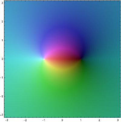
A domain coloring or phase portrait is a popular and attractive way to visualize functions of a complex variable. The absolute value (modulus) of the function at a point is represented by brightness (dark for small modulus, light for large modulus), while the argument (phase) is represented by hue (red for positive real values, yellow-green for positive imaginary values, etc.). This Demonstration creates domain colorings for many well-known functions in complex analysis: trigonometric and exponential functions, Möbius transformations, the Joukowski map, the Koebe function, Weierstrass functions, gamma and beta functions, and the Riemann zeta function.
℘
Details
Details
The terms domain coloring or phase portrait refer to the type of visualization technique for functions of a complex variable used here, or some variation thereof. For a function of a complex variable, each point in the complex plane is colored according to the value of . The brightness represents the absolute value (or modulus) of , with light representing large absolute value and dark representing small absolute value. The hue represents the argument (or phase) of , with red representing positive real numbers, yellow-green representing positive imaginary numbers, cyan representing negative real numbers, and so forth.
f
z
f(z)
f(z)
f(z)
These plots illustrate various phenomena in complex analysis. A dark spot contains a zero of , while a white spot contains a pole. The order of a zero or pole is given by the number of rays of each color emanating from it. Where a single color forms a saddle-shaped region (such as near the point for the function ), the derivative must have a zero. The graphs of and contain essential singularities, and in particular illustrate Picard's great theorem that in any neighborhood of an essential singularity must contain every complex value with at most one exception. Observe that functions such as and the inverse trigonometric functions exhibit branch cuts.
f
π/2+0
sin(z)
1/z
sin(1/z)
f
log
In addition to the standard polynomial, trigonometric, and exponential functions, we have included: the Möbius transformation , the Joukowski map , the Koebe function , a few instances of the beta functions (a,b)dt, the gamma functions and , and the Weierstrass ℘ functions defined by if , and finally the famous Riemann zeta function , defined as the analytic continuation of the Dirichlet series for .
(1-z)/(1+z)
z+1/z
z
2
(1-z)
Β
z
z
∫
0
a-1
t
b-1
(1-t)
Γ(z)=dt
∞
∫
0
z-1
t
-t
e
Γ(a,z)=dt
∞
∫
z
a-1
t
-t
e
℘(u;,)
g
2
g
3
℘(z;,)=x
g
2
g
3
zdt
x
∫
∞
-1/2
4-t-
3
t
g
2
g
3
ζ(z)
∞
∑
k=1
-z
k
Re(z)>1
References
References
[1] E. Wegert, Visual Complex Functions: An Introduction with Phase Portraits, Basel: Birkhäuser/Springer Basel AG, 2012.
[2] A. Sandoval-Romero and A. Hernández-Garduño, "Domain Coloring on the Riemann Sphere," The Mathematica Journal, 2015. doi:10.3888/tmj.17-9.
External Links
External Links
Permanent Citation
Permanent Citation
Matthew Romney
"Domain Coloring for Common Functions in Complex Analysis"
http://demonstrations.wolfram.com/DomainColoringForCommonFunctionsInComplexAnalysis/
Wolfram Demonstrations Project
Published: March 2, 2016