This notebook series is designed to introduce selected dynamic economic models to both advanced undergraduate and graduate students. Economists have relied on a series of economic models to better understand the otherwise highly complex causal relationship among many economic variables. Dynamic economic models set up by systems of either difference or differential equations are particularly useful in tracing the change in the quantity of unknown economic variables (e.g., the capital stock, demand for labor, aggregate output, etc.) and their interactions over time.
This notebook series aims to help students better understand the depth, usefulness, and limitations of major existing micro and macroeconomic models by demonstrating how we can use Wolfram Mathematica to replicate and reconstruct the core ideas and find dynamic solution of the model.
The model introduced in this notebook series include, among others, (1) the cobweb model of the quantity and price adjustment, (2) Keynes’s aggregate demand model, (3) Hicks’s ISLM model, (4) Samuelson’s investment accelerator model, (5) Kalecki’s investment delay model, (6) the predator-prey interaction model, (7) the epidemic model, (8) Ricardo’s three dimensional business cycle model, (9) Marx-Goodwin business cycle and growth model, (10) Smith’s and Ricardo’s growth model, (11) the Harrod-Domar growth model, (12) the Solow growth model, (13) the RBC model, (14) Romer’s new growth model, and (15) the circuit of capital model.
The Cobweb Model of the Price Adjustment II
Introduction
Introduction
As a continuation of the dynamic model of supply and demand, we introduce an expectation variable that affects the interaction between the quantity supplied and the quantity demanded. Here, the term ‘expectation’ is specifically about the future supply price of the product. The producer-seller forms his/her expectation about the future price, and this expected price of the product affect the same producer-seller’s current price setting decision.
Economists have made various attempts to specify how the producer-seller forms the expectation, and we test (1) naive expectation, (2) normal price expectation, and (3) adaptive expectation to see this expectation variable induces some qualitative changes in the behavior of the equilibrium price adjustment. As in the previous Cobweb model of the price adjustment without expectation, the producer-seller of the product must set the current price of the product in response to the change in the price of the product measured previous time periods. The prices of the product measured in the past help the producer-seller form a certain expectation about the desirable price of the product, and it will affect his/her current price setting decision.
Naive expectation
Naive expectation
The first expectation formation is the case when the producer sets the price of the product at time t based upon the existing price of the product at time t-1. The producer-seller of the product expects that the current price of the product will be the same as that measured one time period earlier. The relevant equation for the quantity supplied is then defined as:
In[]:=
Clear[Q,P,Pe,d0,d1,s0,s1,t];Q[t]==d0-d1P[t];Q[t]==s0+s1Pe[t]/.Pe[t]->P[t-1];
The expression “/. Pe[t] -> P[t-1]” is an operation to replace Pe[t] variable with P[t-1] where the notation Pe[t] represents the expected price at time t.
Using the equilibrium condition for this product market, which is Qd[t] = Qs[t], we get P[t] = - :
d0-s0
d1
s1P[t-1]
d1
In[]:=
Solve[d0-d1P[t]==s0+s1P[t-1],P[t]]
Out[]=
P[t]
d0-s0-s1P[-1+t]
d1
This is a linear first-order difference equation, whose solution can be found by using RSolve[ ] function:
In[]:=
?RSolve
Out[]=
In[]:=
RSolve[{d0-d1P[t]==s0+s1P[t-1]},P[t],t]//ExpandAll
Out[]=
P[t]--++
d0
d1+s1
s0
d1+s1
d0
t
-
s1
d1
d1+s1
s0
t
-
s1
d1
d1+s1
-1+t
-
s1
d1
1
Notice that this solution is exactly the same as what we saw in the previous notebook(“The Cobweb Model of the Price Adjustment”). Depending on the relative size of the ratio of s1 and d1, the solution curve can either converge to or diverge away from the steady state value, -.
d0
d1+s1
s0
d1+s1
Normal price expectation
Normal price expectation
The core idea and analytical solution
The core idea and analytical solution
In the normal price expectation, the price expectation variable, Pe[t] is defined as the past price of the product plus the adjustment of this past price toward the normal price level, denoted by Pn. If the past price is different from this normal average price level, the producer-seller adjusts the price at time t according to a certain speed of adjustment, α (0 < α <1).
In[]:=
Clear[Q,P,Pn,Pe,d0,d1,s0,s1,α,t];Q[t]==d0-d1P[t];Q[t]==s0+s1Pe[t]/.Pe[t]->P[t-1]+α(Pn-P[t-1]);
The equilibrium condition in this product market yields the following first-order linear difference equation, whose solution can be found by the same RSolve [] as follow:
In[]:=
RSolve[{d0-d1P[t]==s0+s1(α(Pn-P[-1+t])+P[-1+t])},P[t],t]
Out[]=
P[t]-+
1-(-d0+s0+Pns1α)
t
s1(-1+α)
d1
d1+s1-s1α
-1+t
s1(-1+α)
d1
1
Here, Pn can be perceived as the average price of product measured in the past. If Pn is equal to the steady state value of the equilibrium price of the original supply and demand equation, the solution becomes:
In[]:=
RSolve[{d0-d1P[t]==s0+s1(α(Pn-P[-1+t])+P[-1+t])/.Pn->(s0-d0/d1-s1)},P[t],t]
Out[]=
P[t]+
1-(d0d1-d1s0+d0s1α-d1s0s1α+d1α)
t
s1(-1+α)
d1
2
s1
d1(d1+s1-s1α)
-1+t
s1(-1+α)
d1
1
The case when α = 0.8
The case when α = 0.8
Now suppose that the adjustment parameter is α = 0.8. If d0=4, d1=1.7, s0=0.5, s1=1.1, and P[0]=1, the numerical solution to the normal price expectation equation becomes:
In[]:=
Clear[sol1];d0=4;d1=1.7;s0=0.5;s1=1.1;α=0.8;RSolve[{d0-d1P[t]==s0+s1(α(Pn-P[-1+t])+P[-1+t])/.Pn->(s0-d0/d1-s1),P[0]==1},P[t],t]
Out[]=
{{P[t]0.0117647(-269.99+269.99+85.)}}
-1.t
85.
t
(-11.)
t
85.
t
(-0.129412)
1.t
85.
In[]:=
DiscretePlot0.011764705882352941`-269.9895833333333`+269.9895833333333`+85.`,{t,0,10},PlotRange->Full,AxesLabel->{"time","P[t]"}
-1.`t
85.`
t
(-11.`)
t
85.`
t
(-0.12941176470588237`)
1.`t
85.`
Out[]=
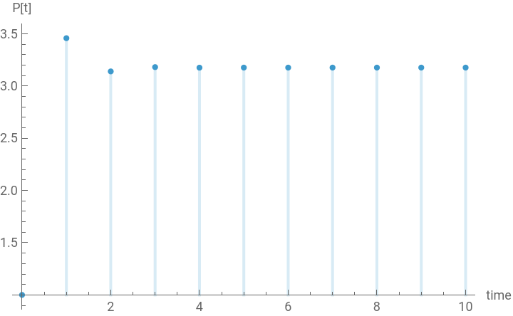
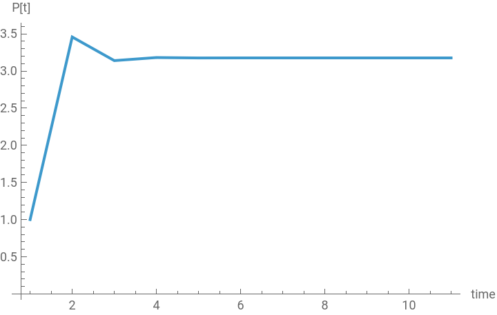
Using the same parameter values, we can also use another built-in function, RecurrentTable[ ] and ListLinePlot[ ]
In[]:=
?RecurrenceTable
Out[]=
In[]:=
?ListLinePlot
Out[]=
In[]:=
d0=4;d1=1.7;s0=0.5;s1=1.1;α=0.8;sol1=RecurrenceTable[{d0-d1P[t]==s0+s1(α(Pn-P[-1+t])+P[-1+t])/.Pn->(s0-d0/d1-s1),P[0]==1},P,{t,0,10}]
Out[]=
{1.,3.45799,3.1399,3.18106,3.17574,3.17643,3.17634,3.17635,3.17635,3.17635,3.17635}
In[]:=
ListLinePlot[sol1,PlotRange->Full,AxesLabel->{"time","P[t]"}]
Out[]=
The case when α = 0.2
The case when α = 0.2
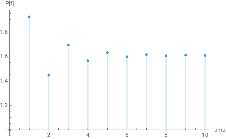
Suppose this time that the price adjustment parameter α = 0.2, while all other parameters and initial value remain the same as before. Then the behavior of the solution curve will be changed as follow:
In[]:=
d0=4;d1=1.7;s0=0.5;s1=1.1;α=0.2;RSolve[{d0-d1P[t]==s0+s1(α(Pn-P[-1+t])+P[-1+t])/.Pn->(s0-d0/d1-s1),P[0]==1},P[t],t]
Out[]=
{{P[t]-0.60839(-2.64368+1.)}}
t
(-0.517647)
In[]:=
DiscretePlot-0.608390332877337`(-2.6436816069554787`+1.`),{t,0,10},PlotRange->Full,AxesLabel->{"time","P[t]"}
t
(-0.5176470588235295`)
Out[]=
In[]:=
d0=4;d1=1.7;s0=0.5;s1=1.1;α=0.2;sol2=RecurrenceTable[{d0-d1P[t]==s0+s1(α(Pn-P[-1+t])+P[-1+t])/.Pn->(s0-d0/d1-s1),P[0]==1},P,{t,0,10}]
Out[]=
{1.,1.92332,1.44537,1.69278,1.56471,1.631,1.59668,1.61445,1.60525,1.61001,1.60755}
In[]:=
ListLinePlot[sol2,PlotRange->Full,AxesLabel->{"time","P[t]"}]
Out[]=
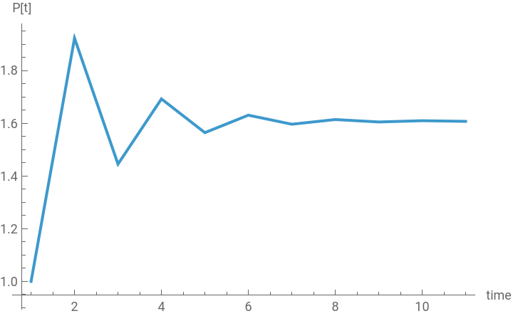
As these two numerical examples illustrate, the higher the value of α, the faster the adjustment of the equilibrium price toward its steady state value.
Adaptive price expectation
Adaptive price expectation
The core idea and analytical solution
The core idea and analytical solution
Suppose that the producer-seller’s price expectation at time t is expressed by Pe[t] = P[t-1] - ρ (P[t-1] - P[t-2]). This expression means that the suppliers use the information about P[t-1] and the price change over the previous two period P[t-1] - P[t-2] to set the current period price. The parameter ρ represents how the supplier responds to the price difference in the previous two time periods.
The mathematical equation and its analytical solution can be found by:
Notice that the equilibrium equation is no longer a first-order difference equation; instead we have a linear second-order difference equation whose solution involving two arbitrarily generated constants of integration.
The case when ρ = 0.8
The case when ρ = 0.8
Suppose the adjustment parameter is ρ = 0.8. Suppose also that we have d0=4, d1=1.7, s0=0.5, s1=1.1, and P[0]=1 and P[1] = 1.2. The numerical solution to this second-order difference equation becomes:
The case when ρ = 0.2
The case when ρ = 0.2
Suppose now that the adjustment parameter is ρ = 0.2. Assuming that all other parameters and the initial values remain the same as before, we get the following numerical solution:
Unlike the normal price expectation case, the higher value of the adjustment parameter ρ induces a greater fluctuation in the solution curve converging toward the steady state value. This greater fluctuation primarily comes from the nature of the second-order difference equation.
Conclusion
Conclusion
We can transform the standard Cobweb model of supply and demand into the one, in which the producer and seller is setting the current price of the product based upon his or her expectation. Though there are many different ways of specifying and modeling this price expectation formation, the resulting supply and demand model would become either the first-order or second-order difference/differential equation.
In this note, we have learned how to incorporate the naive expectation, the normal price expectation, and the adaptive expectation into the original Cobweb model of the equilibrium price adjustment.
One immediate extension of the above discussion is to introduce a nonlinear supply equation and to see the dynamic interaction between the two interrelated product markets when the producer-seller continue to set the price of his/her product based upon their expectation about the desirable price. We can also continue to explore the possibility of integrating the inventory management-workforce adjustment model to this expectation-based Cobweb model of the price adjustment.
Reference
Reference
Giancharlo Gandolfo, Economic Dynamics, Springer: 2010, pp.37-45.
Ronald Shone, An Introduction to Economic Dynamics, Cambridge University Press: 2001, pp.35-38.
Srinivas Raghavendra and Petri T. Piiroinen, An Introduction to Economic Dynamics - Modelling, Analysis and Simulation, Routledge: 2023, pp.33-45.
CITE THIS NOTEBOOK
CITE THIS NOTEBOOK
Introduction to dynamic economic models: the Cobweb model of the price adjustment II
by Hee-Young Shin
Wolfram Community, STAFF PICKS, December 8, 2025
https://community.wolfram.com/groups/-/m/t/3587756
by Hee-Young Shin
Wolfram Community, STAFF PICKS, December 8, 2025
https://community.wolfram.com/groups/-/m/t/3587756