I found the visualization of a complex number problem very appealing in Tsing-hua University (Top 1 college in PRC) for its Elite student selection exam 2021. I use the geometric interpretation for complex plot and encode the related lines in the graphics with the value of target function with Hue function. The result is flamboyant modern art deco.
Problem
Problem
Given a complex number with , find the extreme values of .
z
|z|=1
(z-1)
2
(z+1)
Analysis
Analysis
We use the geometric interpretation of the complex number with unit length: . If you are only interested in the absolute value of the target function, Plot function is adequate in this case:
z=cos(t)+sin(t)
In[]:=
Plot[Abs[((Cos[t]+Sin[t]*)-2)*((Cos[t]+Sin[t]*)+1)^2],{t,-π,π}]
Out[]=
AbsArgPlot also shows the phase variation with respect to :
t
In[]:=
AbsArgPlot[((Cos[t]+Sin[t]*)-2)*((Cos[t]+Sin[t]*)+1)^2,{t,-π,π},PlotLegends->Automatic]
Out[]=
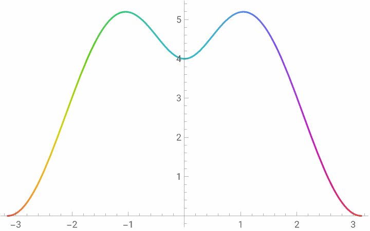
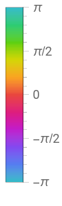
We can define a optimization function friendly function by using the geometric representation of
In[]:=
f[t_]:=EuclideanDistance[{Cos[t],Sin[t]},{2,0}]*EuclideanDistance[{Cos[t],Sin[t]},{-1,0}]^2
Find the exact range of the function:
In[]:=
Maximize[f[t],t]
Out[]=
3
3
,tπ
3
In[]:=
Minimize[f[t],t]
Out[]=
{0,{tπ}}
Animation
Animation
Let’s generate one frame first. The black circle indicates the domain for . The color of each line (connecting to -2 and 1 on complex plane) is encoded with the normalized value of defined above plus a shift parameter ( 0.5 in this case):
z
z
f(t)
In[]:=
GraphicsReverse@TableHuef[t]3
3
+0.5,Line[{{-1,0},{Cos[t],Sin[t]},{2,0}}],{t,Subdivide[-π,π,30]},Thick,Circle[]Out[]=
Changing the shift value in Hue function to create the beautiful animation with more dense lines :
In[]:=
ManipulateGraphicsReverse@TableHuef[t]3
3
+h,Line[{{-1,0},{Cos[t],Sin[t]},{2,0}}],{t,Subdivide[-π,π,120]},Thick,Circle[],{{h,0.24},0,0.9},SaveDefinitions->TrueOut[]=


Changing the radius of z
Changing the radius of
z
The value of the target function changes with respect to enlarged circle for :
z
In[]:=
Plot[Evaluate[Table[Abs[(r*(Cos[t]+Sin[t]*)-2)*(r*(Cos[t]+Sin[t]*)+1)^2],{r,1,5,0.5}]],{t,-π,π},PlotLegends->Table[Row[{"r = ",r}],{r,1/2,5,1/2}]]
Out[]=


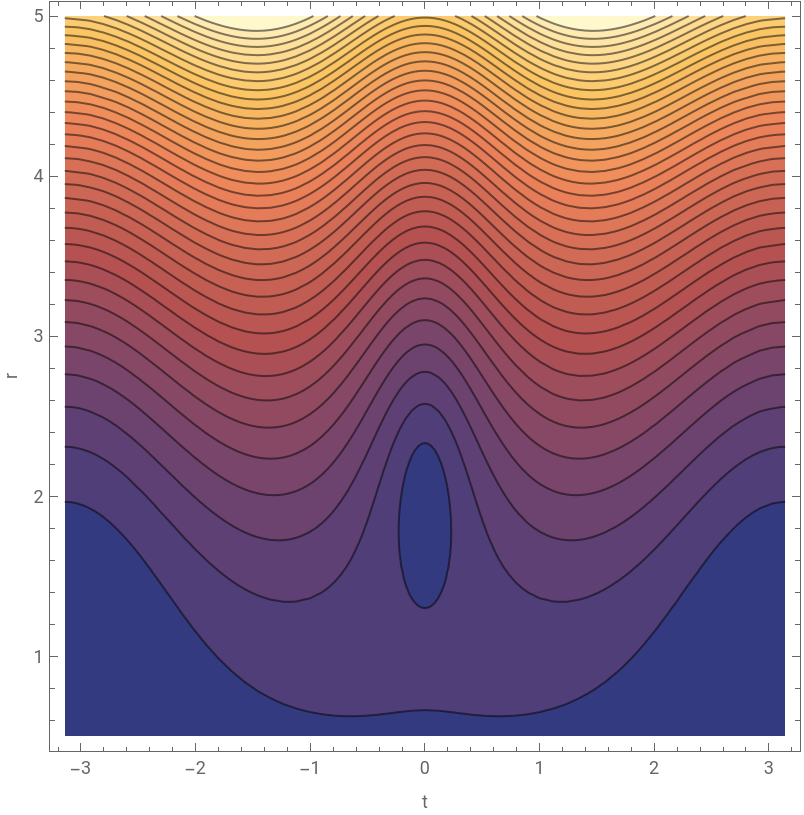
Or use contour plot to show constant given r and t:
f(t)
In[]:=
g[t_,r_]:=EuclideanDistance[r*{Cos[t],Sin[t]},{2,0}]*EuclideanDistance[r*{Cos[t],Sin[t]},{-1,0}]^2
In[]:=
ContourPlot[g[t,r],{t,-π,π},{r,1/2,5},FrameLabel->{"t","r"},Contours->36]
Out[]=
Now we can create animation by changing two variables:
In[]:=
Manipulate[boundary={FindMaxValue[g[t,r],{t,π/3}],Min[FindMinValue[g[t,r],{t,0}],FindMinValue[g[t,r],{t,π}]]}//Quiet;Graphics[{Reverse@Table[{Hue[Rescale[g[t,r],boundary]+h],Line[{{-1,0},r*{Cos[t],Sin[t]},{2,0}}]},{t,Subdivide[-π,π,120]}],Thick,Circle[{0,0},r]},ImageSize->{400,400}],{r,1/2,4},{h,0,1}]
CITE THIS NOTEBOOK
CITE THIS NOTEBOOK
Visualization of a complex number problem with extreme values
by Shenghui Yang
Wolfram Community, STAFF PICKS, May 8 2023
https://community.wolfram.com/groups/-/m/t/2916186
by Shenghui Yang
Wolfram Community, STAFF PICKS, May 8 2023
https://community.wolfram.com/groups/-/m/t/2916186