ABSTRACT (original article): The violation of Bell type inequalities in quantum systems manifests that quantum states cannot be described by classical probability distributions. Yet, Bohmian mechanics is a realistic, non-local theory of classical particle trajectories that is claimed to be indistinguishable by observations from more traditional approaches to quantum mechanics. We set up a spatial version of the GHZ system with qubits realised as positional observables that demonstrates that the Bohmian theory fails to match predictions of textbook quantum mechanics (and most likely experients) unless enlarged by a microscopic theory of collapse of the wave function after observation. For this discrepancy to occur it is essential that positions at different times do not commute. CITATION (original article): Robert C. Helling (2025), Bohmian Mechanics fails to compute multi-time correlations, arXiv:2502.14449. https://doi.org/10.48550/arXiv.2502.14449
In this project we want to compute correlations of positions of particles at different times and compare those to similar expression from Bohmian Mechanics . Everything takes place in the form of particles in box, so the Hilbert space consists of factors of L^2 ([-Pi/2, Pi/2]) . We are mainly interested in the two - dimensional sub - space spanned by be the ground state (denoted g below) and the first excited state (denoted e) . Our main observable tests if the particle is in the left or in the right half of the box and can be written as the sign function in positions space . We denote it by σ below . This is the expression at time zero but to make things interesting, we also need this observable at later times (which we will compute in the Heisenberg representation) .
The time evolution of the two eigenfunctions g and e is simply by multiplication of a phase, but non - trivial linear combinations evolve in more complicated ways. For the Bohmian evolution we have to take particles whose initial positions are distributed according to Abs[ψ]^2 and which then follow the flow of the velocity field given by the imaginary part of the gradient of ψ divided by ψ .
The time evolution of the two eigenfunctions g and e is simply by multiplication of a phase, but non - trivial linear combinations evolve in more complicated ways. For the Bohmian evolution we have to take particles whose initial positions are distributed according to Abs[ψ]^2 and which then follow the flow of the velocity field given by the imaginary part of the gradient of ψ divided by ψ .
The GHZ wave function
In[]:=
ghz[x_,y_,z_]:=(e[x]e[y]e[z]-g[x]g[y]g[z])/Sqrt[2]
Applying the observable swaps symmetric and anti - symmetric wave functions (and actually leaks a bit into higher modes)
In[]:=
sigma[psi_,x_]:=((psi/.e[x]h)/.g[x]8/3/Pie[x])/.h8/3/Pig[x]
Same as an operator
In[]:=
sigma[x_]:=(psisigma[psi,x])
Time evolution, we can ignore a common time dependent phase of g and e
In[]:=
U[psi_,t_]:=(psi/.e[arg_]Exp[3/2It]et[arg])/.et[arg_]e[arg]
Same as an operator
In[]:=
U[t_]:=(psiU[psi,t])
The EPR pair as a test case
In[]:=
epr[a_,b_]=(e[a]g[b]-g[a]e[b])/Sqrt[2]
Out[]=
-e[b]g[a]+e[a]g[b]
2
Range for plots and integrals.
In[]:=
range[a_]:=Evaluate[{a,-Pi/2,Pi/2}]
Test case of correlation from Bohmian Angels paper
In[]:=
Integrate[U[sigma[U[sigma[U[epr[a,b],s],a],t-s],b],-t]epr[a,b]/.{e[c_]Sin[2c],g[c_]Cos[c]},range[a],range[b]]
Out[]=
-Cos
16
9
3(s-t)
2
Heisenberg operator
In[]:=
sigma[ψ_,a_,t_]:=U[sigma[U[ψ,t],a],-t]
... same as an operator
In[]:=
sigmat[a_,t_]:=(psisigma[psi,a,t])
In[]:=
Integrate[sigma[sigma[epr[a,b],b,s],a,t]epr[a,b]/.{e[c_]Sin[2c],g[c_]Cos[c]},range[a],range[b]]
Out[]=
-Cos
16
9
3(s-t)
2
Replacement of ground and excited states with actual wave functions
In[]:=
funcrules={e[arg_]Sin[2arg]Sqrt[2/Pi],g[arg_]Cos[arg]Sqrt[2/Pi]}
Out[]=
e[arg_]Sin[2arg],g[arg_]Cos[arg]
2
π
2
π
(2d expectation value
In[]:=
ev[op_,ψ_]:=Integrate[Evaluate[ComplexExpand[Conjugate[ψ]op[ψ]/.{e[c_]Sin[2c]Sqrt[2/Pi],g[c_]Cos[c]Sqrt[2/Pi]}]],range[a],range[b]]
3d expectation value
In[]:=
ev3[op_,ψ_]:=Integrate[Evaluate[ComplexExpand[Conjugate[ψ]op[ψ]/.{e[x_]Sin[2x]Sqrt[2/Pi],g[x_]Cos[x]Sqrt[2/Pi]}]],range[a],range[b],range[c]]
In[]:=
ev1[op_,ψ_]:=Integrate[Evaluate[ComplexExpand[Conjugate[ψ]op[ψ]/.{e[c_]Sin[2c]Sqrt[2/Pi],g[c_]Cos[c]Sqrt[2/Pi]}]],range[a]]
Again the EPR test case
In[]:=
ev[sigma[sigma[#,a,t],b,s]&,epr[a,b]]
Out[]=
-
64Cos
3(s-t)
2
9
2
π
In[]:=
ev[sigma[sigma[#,a,t],d,s]&,epr[a,b]]
Out[]=
0
In[]:=
ev[#&,epr[a,b]]
Out[]=
1
In[]:=
ev[sigmat[a,t]@*sigmat[b,s],epr[a,b]]
Out[]=
-
64Cos
3(s-t)
2
9
2
π
In[]:=
ev3[#&,ghz[a,b,c]]
Out[]=
1
This is the GHZ correlation we are looking for. It's X at time 0 and Y at time π/2
In[]:=
ev3[sigmat[a,t]@*sigmat[b,s]@*sigmat[c,w],ghz[a,b,c]]
Out[]=
-
512Cos(s+t+w)
3
2
27
3
π
Just make sure, the two and one point functions vanish
In[]:=
ev3[sigmat[a,t]@*sigmat[b,s],(g[a]g[b]g[c]-e[a]e[b]e[c])/Sqrt[2]]
Out[]=
0
In[]:=
ev3[sigmat[a,t],(g[a]g[b]g[c]-e[a]e[b]e[c])/Sqrt[2]]
Out[]=
0
But of course the wave function is normalized
In[]:=
ev3[#&,ghz[a,b,c]]
Out[]=
1
Probabilities at time π/3
In[]:=
DensityPlot3D[Abs[Evaluate[U[t]@ghz[y1,y2,y3]/.funcrules/.tPi/3]^2],Evaluate[range[y1]],Evaluate[range[y2]],Evaluate[range[y3]]]
Out[]=

Probabilities at time 0
In[]:=
DensityPlot3D[Abs[Evaluate[U[t]@ghz[y1,y2,y3]/.funcrules/.t0]^2],{y1,-Pi/2,Pi/2},{y2,-Pi/2,Pi/2},{y3,-Pi/2,Pi/2}]
Out[]=

Pre-compute the probability density
In[]:=
wf=Abs[Evaluate[U[t]@ghz[x,y,z]/.funcrules]]
Out[]=
Abs-+
2
2
Cos[x]Cos[y]Cos[z]3/2
π
2Sin[2x]Sin[2y]Sin[2z]
2
9t
2
3/2
π
2
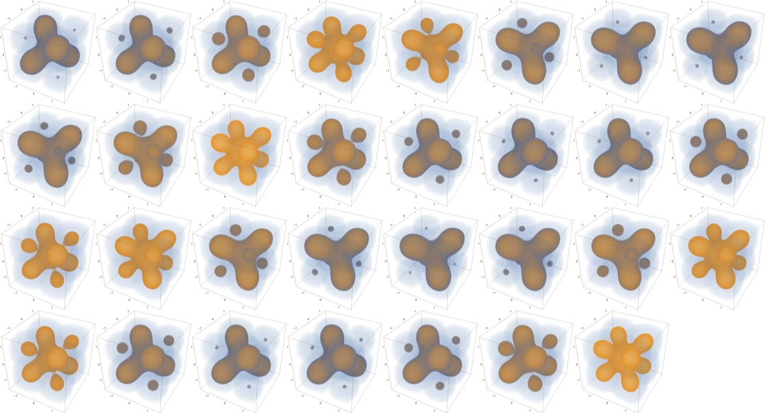
Time evolution as a comic
In[]:=
Table[DensityPlot3D[Evaluate[wf^2],{x,-Pi/2,Pi/2},{y,-Pi/2,Pi/2},{z,-Pi/2,Pi/2}],{t,0,Pi,Pi/3/10}]
In[]:=
ImageCollage[%,BackgroundWhite]
Out[]=
Let's assemble the guiding equation. First compute one component of the velocity field (remember the whole set-up is invariant under permutations of the three particles)
Write the guiding equation with correct coordinate names
Now, we need to set up the initial conditions. Pick points from the wv^2 distribution. Mathematica cannot do this in more than one dimension so we have to do it step by step. This takes some time, so we don't do it in initialization cells to keep start up time reasonable.
First pick x coordinates
Then pick y coordinates from dependent probability
Finally pick also the z coordinates in a similar way
Numerically integrate the guiding equation
Let's plot the expectation value against the mean of the trajectories as a function of time
Here the same, but keep one time fixed at 0
Now for the Frauchinger- Renner Appendix
The state is given in terms of
The state is given in terms of
For the if...then clauses we need projection operators on certain outcomes. All expressions in the paper are expectation values of products of two such projectors. The following is this expectation value taken for measurements at times s and t and projecting to outcomes v and w.
For the Frauchinger - Renner argument we need two qubits and express the state in various bases . Let’ s denote the σx eigenstates as left and right and the σy eigenstates as fro and ba for front and back . Here are the conversion functions . The argument is a dummy which denotes the first (L) and second (R) tensor factor .
Make sure this works as expected :
We can apply this to the Frauchinger - Renner state :
CITE THIS NOTEBOOK
CITE THIS NOTEBOOK
Bohmian mechanics fails to compute multi-time correlations
by Robert Helling
Wolfram Community, STAFF PICKS, March 28, 2025
https://community.wolfram.com/groups/-/m/t/3434706
by Robert Helling
Wolfram Community, STAFF PICKS, March 28, 2025
https://community.wolfram.com/groups/-/m/t/3434706