ORIGINAL DEMONSTRATION: Klaus von Bloh (2011), Peregrine Soliton with Controllable Center in the Causal Interpretation of Quantum Mechanics, Wolfram Demonstrations Project. http://demonstrations.wolfram.com/PeregrineSolitonWithControllableCenterInTheCausalInterpretat/
An analytic and integrable example from a nonlinear Schrödinger equation (NLS) is chosen to visualize the complete way of calculation the trajectories from a wavefunction in the de Broglie - Bohm approach. The article is based on the Wolfram Demonstration “Peregrine Soliton with Controllable Center in the Causal Interpretation of Quantum Mechanics”.
1. Introduction
1. Introduction
The causal interpretation of quantum theory, often called Bohmian mechanics, is an interpretation of quantum mechanics that was developed by Louis de Broglie and David Bohm. This interpretation suggests that particles in the quantum world are described not only by probability waves but also by hidden variables that completely determine the position and momentum of a single particle. Bohm' s interpretation suggests that quantum phenomena are controlled by "pilot waves" at a deeper level of reality, which guide the motion of particles . These pilot waves are deterministic and determine the future state of a particle.
In de Broglie–Bohm theory, the particle has a well - defined trajectory in configuration space calculated from the total phase function. An appealing feature of the Bohmian description is that one can impose initial positions for the trajectories, just as in any classical dynamical system, in which the final positions of the particles are determined by their initial positions. Such initial positions are not controllable by the experimenter, so there is an appearance of randomness in the pattern of detection. So, in conclusion the pilot waves are deterministic, but the particles paths are not controllable because of the uncontrollability of the initial positions [3].
To demonstrate how the Bohmian approach can be applied to other differential equations, an example from nonlinear wave mechanics is used. The commonality lies in the fact that both equations obey the continuity equation.
A Peregrine soliton appears often in nonlinear wave mechanics, in which a nonlinear wave has energy concentrated in a localized oscillatory manner. This article deals with the complete derivation of the trajectory equation in the de Broglie-Bohm interpretation from quantum mechanics. The causal interpretation of quantum theory introduced trajectories that are guided by a quantum potential. The velocities of single particles, following the trajectories, are determined by the phase of the wavefunction. Here, the system is time reversible. A Peregrine soliton of the self-focusing nonlinear Schrödinger (NLS) equation , with = and so on, also known as the Gross–Pitaevskii equation in the causal interpretation is studied. Here the common standard notation is used, where is the temporal and is the spatial coordinate.To emphasize the significance of the Bohmian interpretation, the probability function is consistently referred to as the density function.Use the following command, if you need to save/export graphs created by Mathematica into the current notebook directory:
iψ-ψ+(ψ)ψ=0
∂
t
1
2
∂
x,x
*
ψ
∂
t
∂
∂ t
t
x
In[]:=
SetDirectory[NotebookDirectory[]]
Out[]=
I:\KlausMemory
2. Gross–Pitaevskii equation or Non-linear Schrödinger Equation (NLS)
2. Gross–Pitaevskii equation or Non-linear Schrödinger Equation (NLS)
The focusing nonlinear Schrodinger (NLS) equation is commonly considered as a classic model to describe rogue waves.
In[]:=
NLS[Psi_,PsiC_]:=Psi+IPsi+(PsiPsiC)PsiCE[Prob_,Sx_]:=Prob+(ProbSx)
∂
{x,2}
∂
t
∂
t
∂
x
where is a complex function and (=PsiC) is its complex conjugate. It has a rich of many exact solutions due to its integrability, the Peregrine soliton [1] with controllable center [2] is one of the famous.
ψ
*
ψ
In[]:=
Psi[x_,t_]=Exp[It]1-
4(1+2It)
1+2+4
2
(x-x0)
2
t
Out[]=
t
4(1+2t)
1+4+2
2
t
2
(x-x0)
The complex conjugate yields
*
ψ
In[]:=
PsiC[x_,t_]=Psi[x,t]/.Complex[0,n_]->-Complex[0,n]
Out[]=
-t
4(1-2t)
1+4+2
2
t
2
(x-x0)
To check the correctness, we substitute the solution and its complex conjugate into the Schrödinger equation .
In[]:=
NLS[Psi[x,t],PsiC[x,t]]0//Simplify
Out[]=
True
The wave density function(=squared wavefunction) is given by
In[]:=
Dens[x_,t_]=FullSimplify[ComplexExpand[(Psi[x,t]PsiC[x,t]),TargetFunctions{Re,Im}],Assumptions{Element[_,Reals]}]//Factor
Out[]=
9+40+16-12+16+4+24xx0-32xx0-16x0-12+16+24-16x+4
2
t
4
t
2
x
2
t
2
x
4
x
2
t
3
x
2
x0
2
t
2
x0
2
x
2
x0
3
x0
4
x0
2
(1+4+2-4xx0+2)
2
t
2
x
2
x0
Displaying the density of the squared wavefunction in the - space.
(x,t)
In[]:=
xM=3;time=2;para={x0->1/2};dp=Plot3D[Chop[Dens[x,t]/.para],{x,-xM,xM},{t,-time,time},MeshFalse,ColorFunction"SolarColors",PlotPoints50,PlotRange->All]
Out[]=

3. The Wavefunction in the Polar Form
3. The Wavefunction in the Polar Form
The polar form of the wavefunction is a representation where the wave function is divided into a magnitude factor and a phase factor. The magnitude factor represents the amplitude of the wave function, while the real phase function contains the phase, which could be interpreted as a velocity potential from which the velocity could be derived via the gradient of the phase function.
R
S
S
The amplitude is directly determined by the square root of the density term
R
In[]:=
R[x_,t_]=
Dens[x,t]
//PowerExpand//FullSimplifyOut[]=
16++8(5+2)
4
t
2
(3-2)
2
(x-x0)
2
t
2
(x-x0)
1+4+2
2
t
2
(x-x0)
The phase function gives
In[]:=
S[x_,t_]=ArcTan[ComplexExpand[Im[Psi[x,t]],TargetFunctions{Re,Im}]/ComplexExpand[Re[Psi[x,t]],TargetFunctions{Re,Im}]]//FullSimplify
Out[]=
ArcTan
-8tCos[t]+(-3+4+2)Sin[t]
2
t
2
(x-x0)
(-3+4+2)Cos[t]+8tSin[t]
2
t
2
(x-x0)
The wavefunction in the polar form is given by
In[]:=
Θ[x_,t_]=R[x,t]Exp[IS[x,t]]
Out[]=
ArcTan
-8tCos[t]+-3+4+2Sin[t]
2
t
2
(x-x0)
-3+4+2Cos[t]+8tSin[t]
2
t
2
(x-x0)
16++8(5+2)
4
t
2
(3-2)
2
(x-x0)
2
t
2
(x-x0)
1+4+2
2
t
2
(x-x0)
and its complex conjugate
In[]:=
ΘC[x_,t_]=Θ[x,t]/.Complex[0,n_]->-Complex[0,n]
Out[]=
-ArcTan
-8tCos[t]+-3+4+2Sin[t]
2
t
2
(x-x0)
-3+4+2Cos[t]+8tSin[t]
2
t
2
(x-x0)
16++8(5+2)
4
t
2
(3-2)
2
(x-x0)
2
t
2
(x-x0)
1+4+2
2
t
2
(x-x0)
Check correctness of the formula.
In[]:=
NLS[Θ[x,t],ΘC[x,t]]0//Simplify
Out[]=
True
4. The Velocity of a Single Particle
4. The Velocity of a Single Particle
There are two different ways for calculation the velocity: 1. From the phase function of the wavefunction in the polar form (or eikonal form) 2. From the wavefunction directly via the wave density current .
S
j
To check the correctness of the velocities the continuity equation ρ+(ρv)=0 with is used.
∂
t
∂
x
ρ=
*
ψψ
In[]:=
Sx[x_,t_]=2D[S[x,t],x]//PowerExpand//FullSimplify
Out[]=
64t(x-x0)
16++8(5+2)
4
t
2
(3-2)
2
(x-x0)
2
t
2
(x-x0)
To verify the velocity
In[]:=
CE[Dens[x,t],Sx[x,t]]==0//Simplify
Out[]=
True
The alternative approach directly via the wave density current here, with where the wave density current is defined as: from which the velocity is given by with .
j
j=-(ψ-ψ)
*
ψ
∂
x
∂
x
*
ψ
j
j=vρ
v
v==-ψ-
j
ρ
∂
x
ψ
∂
x
*
ψ
ψ
ρ=
*
ψψ
In[]:=
v[x_,t_]=2ComplexExpand[Im[D[Psi[x,t],x]/Psi[x,t]]]//PowerExpand//FullSimplify
Out[]=
64t(x-x0)
16++8(5+2)
4
t
2
(3-2)
2
(x-x0)
2
t
2
(x-x0)
Which yields the same term as for
Sx
In[]:=
CE[Dens[x,t],v[x,t]]==0//Simplify
Out[]=
True
The Trajectories of Single Particles
The Trajectories of Single Particles
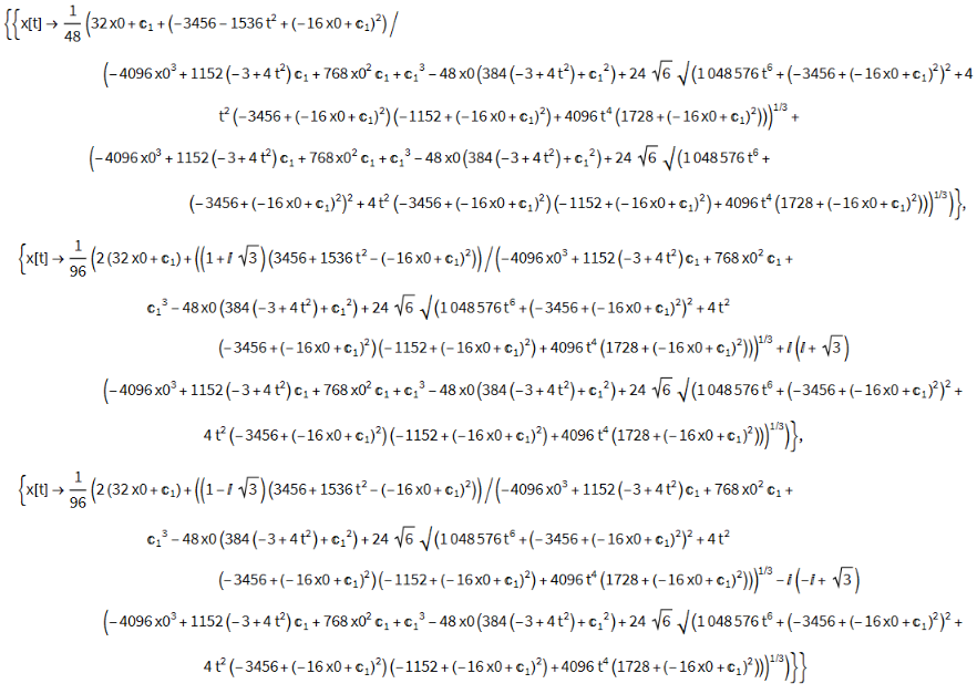
From classical mechanics the path versus time law is obtained by integration the velocity term: (one-dimensional) or =(multi dimensional). This method could be applied to the causal interpretation, only if the conservation of density is given, meaning that the continuity equation is fulfilled.
x=
∫vt
r
∫t
v
The integration with respect to time leads to the following analytical solutions.
In[]:=
sol=DSolve[x'[t]v[x[t],t],x[t],t]//FullSimplify
Here, only the real valued function is used
The initial positions are
Here the plot with the analytic function
Together with the wave density
The numerical solution of the differential equation for the position-time law leads to the same result.
The Quantum Potential
The Quantum Potential
The two key properties are that the QP depends on the form rather than on its magnitude and it needs not fall off with increasing distance.
The quantum potential is defined as
Snapshots
Snapshots
To observe how everything interacts, the density, the velocity field and the quantum potential are displayed together. On the YouTube channel you can see the animation [4].
To save the picture
References
References
[1] D . H . Peregrine, "Water Waves, Nonlinear Schrödinger Equations and Their Solutions," Journal of the Australian Mathematical Society, Series B, 25 (1), 1983 pp . 16–43. journals . cambridge . org/action/displayAbstract?fromPage = online & aid = 3968224.
[2] X . -C . Wang, J . -S . He, and Y . -S . Li, "Rogue Wave with a Controllable Center of Nonlinear Schrödinger Equation," Communications in Theoretical Physics, 56 (4), 2011 pp . 631–637. DOI 10.1088/0253-6102/56/4/06.
[3] P . R . Holland, The Quantum Theory of Motion : An Account of the de Broglie–Bohm Causal Interpretation of Quantum Mechanics, New York : Cambridge University Press, 1993.
[4] K . von Bloh, The Motion of a Peregrine Soliton in the de Broglie Bohm Interpretation of Quantum Mechanic . [Video] . (Jun 20, 2023) https://youtu.be/PZYyErQ-3jg
CITE THIS NOTEBOOK
CITE THIS NOTEBOOK
Nonlinear Schrödinger equation (NLS) in the causal interpretation (de Broglie Bohm theory)
by Klaus von Bloh
Wolfram Community, STAFF PICKS, June 21, 2023
https://community.wolfram.com/groups/-/m/t/2940891
by Klaus von Bloh
Wolfram Community, STAFF PICKS, June 21, 2023
https://community.wolfram.com/groups/-/m/t/2940891