First let’s import a version of the provided model with some descriptions and details added:
In[]:=
model=ImportString,"MO";
Let's keep track of the start and parameter values of interest as integers and rationals. This will be useful for the analytical solution:
In[]:=
parVals={"r"->22,"l"->1/5,"c"->1/100000};initVals={"inductor1.i"->6/5,"capacitor1.v"->24};
Let’s set those parameter and initial values in the model:
In[]:=
model=SetSystemModel[model,<|"ParameterValues"->parVals,"InitialValues"->initVals|>];
Let’s extract the equations of the model with a method that specifies elimination:
In[]:=
eqs=SystemModel[model,"SystemEquations",Method->{"Elimination"->All,"ReduceIndex"->True}];
Further simplifications and eliminations are needed to turn these equations into something that the Wolfram Language (WL) can process easily. Let’s start by eliminating some variables that are not of much interest:
In[]:=
eliminVars=t.,t.,t.,t.,t.,t.,t.,t.,t.,t.,t.,t.;
resistor1.R_actual
resistor1.T_heatPort
resistor1.LossPower
ground1.p.i
switch1.LossPower
switch1.s
switch1.v
switch1.i
switch.LossPower
switch.s
switch.i
switch.v
In[]:=
reducedEquations=List@@Eliminate[eqs,eliminVars]//Simplify
Out[]=
t.+t.t.,(1+(-))t.t.,t.t.,If[,1,]If[,,1]t.+t.+If[,1,]t.+t.+If[,,1]If[,1,]t.+t.-t.0,t.t.,t.t.
capacitor1.i
resistor1.i
inductor1.i
resistor1.R
resistor1.alpha
resistor1.T
resistor1.T_ref
resistor1.i
capacitor1.v
capacitor1.v
Vc
booleanConstant1.k
switch.Ron
booleanConstant2.k
switch1.Goff
capacitor1.v
inductor1.v
booleanConstant2.k
switch1.Ron
capacitor1.i
resistor1.i
booleanConstant1.k
switch.Goff
booleanConstant2.k
switch1.Ron
capacitor1.v
inductor1.v
Vi
capacitor1.i
capacitor1.C
′
capacitor1.v
inductor1.v
inductor1.L
′
inductor1.i
This is already more readable. Let’s set some parameter values to find an even cleaner presentation of the equations in the model:
In[]:=
nonNumPars=Select[SystemModel[model,"ParameterValues"],!MemberQ[{,,},#[[1]]]&]
r
c
l
Out[]=
{True,False,,,,300.15,0,,0,0,0,0,,}
k1
k2
inductor1.L
l
capacitor1.C
c
resistor1.R
r
resistor1.T_ref
resistor1.alpha
resistor1.T
resistor1.T_ref
switch.Ron
switch.Goff
switch1.Ron
switch1.Goff
booleanConstant1.k
k1
booleanConstant2.k
k2
In[]:=
reducedEquationsEval=reducedEquations//.nonNumPars;%//TableForm
Out[]//TableForm=
capacitor1.i resistor1.i inductor1.i |
r resistor1.i capacitor1.v |
capacitor1.v Vc |
capacitor1.v inductor1.v |
capacitor1.i c ′ capacitor1.v |
inductor1.v l ′ inductor1.i |
Let’s change variable names to make them more WL-friendly and set the parameters to the values we chose at the start:
In[]:=
wlEqs=reducedEquationsEval/.->Function[t,ci[t]],->Function[t,cv[t]],->Function[t,ii[t]],->Function[t,iv[t]],->Function[t,ri[t]],->Function[t,vc[t]],->r,->c,->l,t.->t/.Thread[{r,l,c}->parVals[[All,2]]]
capacitor1.i
capacitor1.v
inductor1.i
inductor1.v
resistor1.i
Vc
r
c
l
Out[]=
ci[t]+ri[t]ii[t],22ri[t]cv[t],cv[t]vc[t],cv[t]+iv[t]0,ci[t][t],iv[t][t]
′
cv
100000
′
ii
5
Now we can pass this to DSolve, adding the initial conditions that we chose at the start, to find the analytical solution:
In[]:=
initEqs=MapThread[Equal,{{ii[0],cv[0]},initVals[[All,2]]}];sol=DSolve[Join[wlEqs,initEqs],{cv[t],ii[t],ci[t],iv[t],ri[t],vc[t]},t]//First//FullSimplify
Out[]=
ci[t]33870+1113,cv[t],ii[t]33870-717,iv[t]-,ri[t],vc[t]
-(50+
500
11
2258
)t
2258
+(33870-11132258
)1000
2258
t11
620950
121129-30
-(50+
500
11
2258
)t
2258
+(1129+302258
)1000
2258
t11
1129
-(50+
500
11
2258
)t
2258
+(33870+7172258
)1000
2258
t11
56450
121129-30
-(50+
500
11
2258
)t
2258
+(1129+302258
)1000
2258
t11
1129
61129-30
-(50+
500
11
2258
)t
2258
+(1129+302258
)1000
2258
t11
12419
121129-30
-(50+
500
11
2258
)t
2258
+(1129+302258
)1000
2258
t11
1129
Now we only need to simulate the model with a specific simulation method. “Euler” is generally not the default method for simulation but we can pick it in the SystemModelSimulate function. As mentioned by Henrik, this is explicit Euler’s method, no the inverse Euler method. Check the documentation for more details:
https://reference.wolfram.com/language/ref/SystemModelSimulate.html
Notice that we are also free to pick method suboptions like step size, which naturally affects the simulation results. We also pick here a simulation interval from 0 to tMax = 0.04, since most of the difference to the analytical solution seems to appear at the start of the simulation. Notice that for the “Euler” method, the choice of step size can affect substantially the time it takes to finish the simulation for a given time interval:
In[]:=
tMax=0.04;sim=SystemModelSimulate[model,tMax,Method->{"Euler","StepSize"->}];cvSim=sim["capacitor1.v",t];cvDSolve=cv[t]/.sol;absDiff=Abs[cvSim-cvDSolve];
-6
10
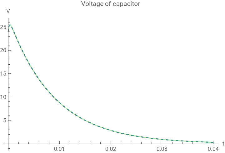
If we plot the two solutions with these specific choices, we notice that it is hard to see the difference at first sight:
In[]:=
Plot[{cvSim,cvDSolve},{t,0,tMax},PlotStyle->{Dashed,Directive[Darker[Green],Opacity[0.3]]},PlotRange->All,PlotLegends->{"Simulation","DSolve"},PlotLabel->"Voltage of capacitor",AxesLabel->{"t",QuantityForm["Volts","Abbreviation"]}]
Out[]=


But we can instead plot the absolute value of the error, here plotted in log scale with LogPlot:
In[]:=
LogPlot[absDiff,{t,0,tMax},PlotRange->All,PlotLabel->"Absolute value of error",AxesLabel->{"t",QuantityForm["Volts","Abbreviation"]}]
Out[]=
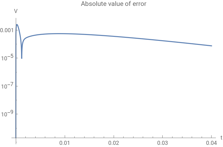
We can also easily find the maximum of the absolute value of the error in the given simulation time interval:
In[]:=
NMaximize[{absDiff,0<=t<=tMax},t]
Out[]=
{0.00253696,{t0.000222008}}
For interesting applications of circuit simulation and the use of System Modeler and Mathematica take a look at these blogs
https://blog.wolfram.com/author/leonardo-laguna-ruiz/
https://blog.wolfram.com/author/leonardo-laguna-ruiz/