A projectile in vacuum takes a perfectly parabolic path as it is only under the influence of the gravity. However, in practice, resistive forces such as drag produce aerodynamical effects on the projectile which alter the path that it moves along . In this project, we will use equations and animations to study the complex relationship between air and a soccer ball and the effect that this relationship has on the path the soccer ball eventually takes.
Ideal Case - Soccer Balls in Vacuum
Ideal Case - Soccer Balls in Vacuum
A soccer ball travelling in vacuum undergoes projectile motion: a specific type of motion in which an external force is applied only at the beginning of the trajectory. Post that, the soccer ball is subject only to gravity. The velocity of the ball can be divided into two components, one horizontal and the other vertical. The vertical component of the velocity is constantly reduced due to the acceleration produced by gravity. In contrast, the horizontal component of the velocity remains constant as there is no force acting in that direction to produce any acceleration. As a result, the ball rises to a maximum height at which its vertical component of the velocity becomes zero. It begins to fall down, following a parabolic path. We define initial values for these conditions.
Defining initial velocity of the soccer ball in metres per second
In[]:=
initialVelocity = 30;
Defining the launch angle of the soccer ball with the ground in degrees
In[]:=
launchAngleDeg = 45;
Defining the value of acceleration due to gravity in metres per second square
In[]:=
g = 9.81;
Converting the launch angle from degrees to radians
In[]:=
launchAngleRad = launchAngleDeg * Pi/180;
Next, we use kinematic equations to make functions for the displacement of the soccer ball in two dimensions. We can use these equations as the acceleration on the ball remains constant.
Making a function for the displacement of the ball in the X and Y directions
In[]:=
displacementX[t_] := initialVelocity * Cos[launchAngleRad] * tdisplacementY[t_] := initialVelocity * Sin[launchAngleRad] * t - 0.5 * g * t^2
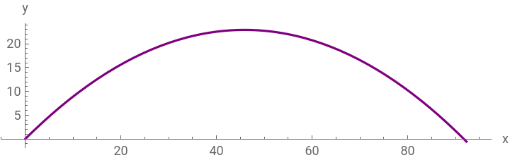
We plot and model the path of the ball to visualize this concept over the entire time period of motion
Plotting a graph for the path of the soccer ball
In[]:=
ParametricPlot[{displacementX[t],displacementY[t]},{t,0,4.35},PlotStyle->Purple,AxesLabel->{"x","y"}]
Out[]=
Making a model for the path of the soccer ball
In[]:=
Animate[Show[ParametricPlot[{displacementX[t],displacementY[t]},{t,0,time}],Graphics[{Red,Disk[{displacementX[time],displacementY[time]}]}]],{time,0.00001,(2*initialVelocity*Sin[launchAngleRad])/g},SaveDefinitions->True,AnimationRunning->False]
Out[]=
The animation confirms the perfect parabolic path of the soccer ball. We can see that the ball travels a huge distance of approximately 90 units before coming to rest.
Soccer Balls In Air - Drag Forces
Soccer Balls In Air - Drag Forces
When a soccer ball is travelling in air, it is under the influence of gravity as well as the drag force. Drag is an aerodynamic force which is generated by the interaction of the ball (a solid) with air (a fluid). It acts in a direction opposite to the motion of the ball and works to reduce its speed. Drag on a soccer ball depends on the following factors:
◼
The speed of the ball in the air (v)
◼
The area of the cross section of the ball (A)
◼
The density of the air (rho)
◼
The drag coefficient (Cd)- which depends upon the shape and surface types of the ball.
The formula for drag is given by D = 0.5*v^2*A*rho*Cd
We define some of these variables using experimentally obtained data from NASA and laws that govern the game of soccer. For example, according to FIFA, a soccer ball has to be between 410 and 450 grams at the start of the match. Hence, we have its mass to be equal to 430 grams or 0.43 kilograms.
Defining mass of the ball in kilograms, drag coefficient, air density at room temperature in kilograms per metre cube, and area of cross section of the ball in metres squared.
In[]:=
mass = 0.43;dragCoefficient = 0.25;area = 0.038;airDensity = 1.292;
Here, we make more complex functions that factor in aerodynamic drag into the equations and plot the path of the ball . Please note that for all the following cases:
◼
The ball has no spin on it .
◼
The distance travelled on the graphs will be different than the distance travelled on the animations . This is because the scale on the two is different - graphs are zoomed in and animations track the path of the ball after zooming out.
◼
The wind speeds have been changed across cases for variety.
Defining the equations of motion
In[]:=
equations = xPos''[t]==-dragCoefficient*airDensity*area*(xPos'[t]^2+yPos'[t]^2)*xPos'[t](2*mass), yPos''[t]==-g-dragCoefficient*airDensity*area*(xPos'[t]^2+yPos'[t]^2)*yPos'[t](2*mass), xPos[0]==0, yPos[0]==0, xPos'[0]==initialVelocity*Cos[launchAngleRad], yPos'[0]==initialVelocity*Sin[launchAngleRad];
Solving the equations of motion using differential equations
In[]:=
solution = NDSolve[equations, {xPos[t],yPos[t]}, {t, 0, 1.75}];
Plotting the trajectory of the ball
In[]:=
A1=ParametricPlot[Evaluate[{xPos[t],yPos[t]}/.solution],{t,0,1.75},PlotStyle->Orange,AxesLabel->{"x","y"}]
Out[]=
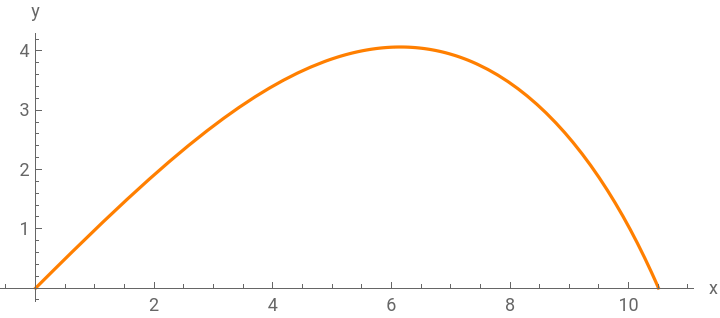
Now, we made a model of the trajectory of the ball using first order differential equations and animation.
Defining the initial velocities in both the X and Y directions in numeric form to plug into the function
In[]:=
VxN = N[initialVelocity * Cos[launchAngleRad]];VyN = N[initialVelocity * Sin[launchAngleRad]];
Writing the differential equation and modelling it
In[]:=
sol = NDSolve[{xPos'[t]==VxN - dragCoefficient * xPos[t] * t, yPos'[t]==VyN - g * t - dragCoefficient * yPos[t] * t,xPos[0] == 0,yPos[0] == 0}, {xPos, yPos}, {t, 0, 3.51}];
In[]:=
p1=Animate[Show[ParametricPlot[{xPos[t],yPos[t]}/.sol[[1]],{t,0,time},AxesLabel->{"x","y"}],Graphics[{Red,Disk[{xPos[time],yPos[time]}/.sol[[1]],0.4]}]],{time,0.0001,3.51},SaveDefinitions->True,AnimationRunning->False]
Out[]=
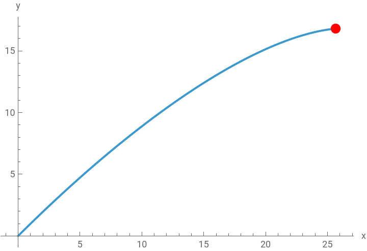
This animation shows us something very interesting. With only the horizontal component of the wind in the negative X direction, the ball comes to rest much faster than in vacuum. After the vertical velocity of the ball becomes zero at the highest point, and it starts falling freely, the resultant vector of the drag force and gravity make the ball fall sharply down. The ball comes to rest after travelling a distance of approximately 30 units. Hence, to make a soccer ball reach the same distance as it would in vacuum, it has to be hit with a much higher initial force.
Varying Wind Speeds And Directions
In this section, we will be considering wind - which is air in motion. We will also be changing the speeds and directions of the wind to make the situation more realistic. Most of the times, the wind in the horizontal direction is faster than the vertical direction as the height of the atmosphere is only a few kilometres. However, both directions are present. Along with this, we will be varying the value of air density in our functions. Air density is inversely proportional to the height of the atmosphere. This means that as we go higher and higher, the air becomes rarer and rarer. Please note that in this section the drag coefficient of air is a constant value, a positive wind speed in X and Y means that the direction of the wind is along the positive X (towards the right)and positive Y (vertically upwards) direction respectively, and a negative wind speed in X and Y means that the direction of the wind is along the negative X(towards the left) and negative Y(vertically downwards) direction respectively.
Case 1
Case 1
Defining wind speed in the X and Y directions in metres per second
Defining scale height for the exponential model of the atmosphere in metres
Defining air density at sea level in kilograms per metre cube
We use the same initial velocity, launch angle, cross sectional area of the ball, etc. for ease of comparison with other cases. Even so, we have to make new equations of motion factoring in the new variables.
Defining the equations of motion
Solving the equations of motion using differential equations
Plotting the trajectory of the ball
To form a model of the path of the soccer ball, we now have to account for the wind direction in our function. We solve the second order differential equation and model the ball’s path.
Defining effect of wind direction using speeds defined above
Writing the differential equation, solving, and animating it
This animation displays the fact that if the wind is blowing in the direction of the motion of the ball in the horizontal direction, and is also simultaneously pushing the ball up in the vertical direction, the ball travels a much farther path than it would in vacuum. The ball travels a distance of approximately 110 units . The concept behind this is the fact that drag is relative to the speed the projectile with respect to the air around it. As mentioned in the above section, with no wind, the drag force is proportional to the square of the velocity of the ball. However, if we take an example of a wind which has a velocity of 6 metres per second in the direction of travel, the drag is proportional to (velocity - 6)^2. This makes the drag force lower and hence the ball travels farther.
Case 2
Case 2
Now, instead of using positive values of wind speeds, we use negative ones with different values to compare the effect.
Defining wind speed in the X and Y directions in metres per second
We use the same values for scale height and sea level air density
Defining the equations of motion
Solving the equations of motion using differential equations
Plotting the trajectory of the ball
Now, we form an animation model for the trajectory.
Defining effect of wind direction using speeds defined above
Writing the differential equation, solving, and animating it
Here, we observe that when the wind is travelling in the negative X and Y directions, the ball is sharply pulled back almost as if it had to return to its original path. It travels a minimal distance of 8 units.
Case 3
Case 3
In this case, we take a positive value of the wind speed in the X direction and a negative value of the wind speed in the Y direction
Defining wind speed in the X and Y directions in metres per second
Defining the equations of motion
Solving the equations using differential equations
Plotting the trajectory of the ball
Defining effect of wind direction using speeds defined above
Writing the differential equation, solving, and animating it
When the direction of the wind is in the positive X and negative Y direction, the ball takes a parabolic path but covers a distance of approximately 45 units. This is lesser than the amount that it covered in vacuum and when both the wind directions were positive. However, it was more than the distance the ball covered in stagnant air.
Case 4
Case 4
For the last case, we take a negative wind speed in the X direction and a positive wind speed in the Y direction
Defining wind speed in the X and Y directions in metres per second
Defining the equations of motion
Solving the equations using differential equations
Plotting the trajectory of the ball
Defining effect of wind direction using speeds defined above
Writing the differential equation, solving, and animating it
When the direction of the wind is in the negative X and positive Y direction, the ball travels in a path that is similar to when both the wind directions are negative. The major difference is in the distance the ball travels. In this case, the ball travels approximately 13.5 units whereas it travelled 8 units in that one. But, we should keep in mind that the speeds of the winds themselves were varied too.
Varying the drag coefficient with velocity
Varying the drag coefficient with velocity
In all the cases above, we used a constant value for drag coefficient that we obtained from experimental NASA data on soccer balls. Nevertheless, as discussed previously, drag force is a variable force. It changes with velocity and is actually directly proportional to the square of the velocity of the ball. This makes the coefficient of drag to be inversely proportional to the square of velocity.
In this section, we will make functions that vary the drag coefficient with the velocity of the soccer ball. In order to do so, we have to define some values. Please note that we will be using positive values for wind speeds in both the X and Y directions.
Defining the diameter of the soccer ball in metres
Defining the approximate value of the dynamic viscosity of air in kilograms per metre second
Defining wind speed in the X and Y directions in metres per second
Making a function for the drag coefficient
Defining the equations of motion
Solving the equations of motion using differential equations
Plotting the trajectory of the ball
Defining effect of wind direction using speeds defined above
Writing the differential equation, solving, and animating it
Comparison Of Graphs
Comparison Of Graphs
This graph combines all the trajectories of the soccer ball when air was involved . We make a key with the color of the path, and the conditions that made that path possible below for easy identification. In order of the longest distance travelled to the shortest distance travelled:
◼
Red - Wind direction was positive in both the X and Y
◼
Green - Wind direction was positive in the X and negative in the Y
◼
Black - Drag coefficient was varied with velocity. Wind direction was positive in both the X and Y
◼
Orange - Drag coefficient was constant and the air was stagnant
◼
Yellow - Wind direction was negative in the X and positive in the Y
◼
Blue - Wind direction was negative in both the X and Y
Spinning Soccer ball - Magnus Effect
Spinning Soccer ball - Magnus Effect
In all the above sections, we considered the ball to have no spin on it. Now, we take a case in which the ball is spinning through the air. This adds a new force on the ball called the Magnus Force - which is the pressure differential that curves the ball gradually. The direction of the Magnus Force is perpendicular to the linear velocity of the ball.
When you hit a soccer ball with the inside of your right foot, it spins in an anticlockwise direction. The ball moving forward exerts a force on the air in the forward direction as well. As a result of Newtons Third Law of Motion, which states that every action has an equal and opposite reaction, the air pushes the ball back in the opposite direction. However, near the ball, there is a thin layer of air that is slowed down and dragged around, due to friction. When the incoming air passes the ball, the side moving in the same direction as the ball is accelerated, follows the curve of the ball and is hence deflected to the right. The incoming air that passes the ball on the side that is moving against the ball is opposed, and moves straight with less speed due to a loss of energy. Therefore, we get a net force of the wind towards the right, and the ball moves left, again in accordance with Newtons Third Law.
When you hit a soccer ball with the outside of your right foot, it spins in a clockwise direction. The same process continues except that this time the net force of the wind is towards the left, and the ball moves right.
A lot of the most famous goals scored in soccer, such as Roberto Carlos’ ‘trivela’ shot with the outside of his cleat, and David Beckham’s ‘banana kick’ with the inside of his cleat, are only possible due to the Magnus Effect.
To visualize the basic difference between the path of a ball with spin and one without spin, we form a parametric plot in 3 dimensions.
Plotting the motion of a ball with spin in red and without spin in green
To understand this 3D plot, we define what the three axes mean in terms of soccer:
◼
The X axis is the goal line (the shorter lines on the rectangular soccer field)
◼
The Y axis is the side line (the longer lines on the rectangular soccer field)
◼
The Z axis is the vertical space above the soccer field
In the graph, we see that both the balls have movement in the Y and Z directions. The difference is that when a ball has spin (red path), it has some movement in the X direction as well. Without spin (blue path), there is no movement in the X direction.
I would like to dive deeper into this case in the future and make equations which factor in this force. Animating these equations in 3D would be a fun extension to this project.
I would like to dive deeper into this case in the future and make equations which factor in this force. Animating these equations in 3D would be a fun extension to this project.
Citations
Citations
◼
NASA . (n . d . -a) . Forces on a soccer ball . NASA . https : // www . grc . nasa . gov/www/k - 12/airplane/socforce . html
◼
3. soccer kick – effects of aerodynamic drag - Brunel University London. (n.d.). https://www.brunel.ac.uk/~spstnpl/LearningResources/SoccerKickLab.pdf
◼
Soccer ball lift coefficients via trajectory analysis. (n.d.-b). https://faculty.lynchburg.edu/goff_j/Goff_Carre_EJP_2010.pdf
◼
Horizontal jumping biomechanics among elite female handball players ... (n.d.-b). https://www.researchgate.net/publication/336349732_Horizontal_jumping_biomechanics_among_elite_female_handball_players_with_and_without_anterior_cruciate_ligament_reconstruction_An_ISU_based_study
Acknowledgement
Acknowledgement
I would like to give a huge thanks to my mentor Athanasios Paraskevopoulos for guiding me throughout this project and teaching me a variety of mathematics and physics concepts. I would also like to thank Karan Chakravarthy, Nora Popescu, and Theodore Moustakas for their help in debugging code and making this entire process even more enjoyable than it already was.
CITE THIS NOTEBOOK
CITE THIS NOTEBOOK
Parabolic perspectives: exploring the diverse trajectories of soccer balls
by Adhiraj Sud
Wolfram Community, STAFF PICKS, July 13, 2023
https://community.wolfram.com/groups/-/m/t/2964070
by Adhiraj Sud
Wolfram Community, STAFF PICKS, July 13, 2023
https://community.wolfram.com/groups/-/m/t/2964070