This project explores how biological neurons encode information through excitability, bifurcation dynamics, and population-level sparsity, and shows that these same principles are fundamental to modern artificial neural networks. Using the FitzHugh-Nagumo (FHN) model, a 2D reduction of the Hodgkin-Huxley equations, we analyze single-neuron phase-plane geometry, characterize the Hopf bifurcation as the mathematical origin of the firing threshold, and derive the neuron’s frequency-input (F-I) curve as its effective transfer function. When extending to small coupled heterogeneous networks, we demonstrate that sparse activity patterns emerge naturally from threshold diversity without any global coordination, and that sparsity is maximized at intermediate connectivity. Finally, we compare the biological F-I curve to the activation functions used in AI (ReLU, etc.) and compare the biological networks with artificial networks.
Introduction
Introduction
Understanding how neurons work requires models that are simple enough to reason with and complex enough to produce interesting behavior. Full biophysical models like Hodgkin-Huxley are highly accurate but involve four coupled equations and are hard to build intuition from. Purely conceptual descriptions go too far the other way, losing the emergent phenomena, like threshold firing and population sparsity, that make neural computation worth studying. This project uses the FitzHugh-Nagumo (FHN) model to bridge that gap: a two-variable system that is easy to simulate and visualize, yet sufficiently rich to capture realistic spiking behavior and network-level coding properties. The key insight is that a neuron’s firing threshold arises naturally from the geometry of its equations, that the relationship between input current and firing rate mirrors the activation functions used in artificial neural networks, and that when you connect many such neurons together with slightly different properties, sparse activity patterns emerge on their own.
The FitzHugh-Nagumo Neuron
The FitzHugh-Nagumo Neuron
The FitzHugh-Nagumo (FHN) model is a 2D simplification of the 4D Hodgkin-Huxley equations. It captures the essential dynamics of neural excitability, which entails of a fast variable v and a slow w. You don’t need all the molecular complexity of ion channels to understand neurons spike. Instead, you need a fast positive feedback (depolarization) and a slow negative feedback (repolarization).We use the FitzHugh-Nagumo Equations: v--w+, which is the fast membrane voltage analog and ϵ(v+a-b*w), which is the slow recover/adaption. Here, the parameters are which are the shape of the w-nullcline, which is the timescale separation, and whichistheexternal input current.
dv
dt
3
v
3
I
ext
dw
dt
a,b
ϵ
I
ext
In[]:=
ClearAll["Global`*"];aDefault=0.7;bDefault=0.8;epsDefault=0.08;fhnV[v_,w_,Iext_]:=v-v^3/3-w+Iext;fhnW[v_,w_,a_,b_,eps_]:=eps*(v+a-b*w);
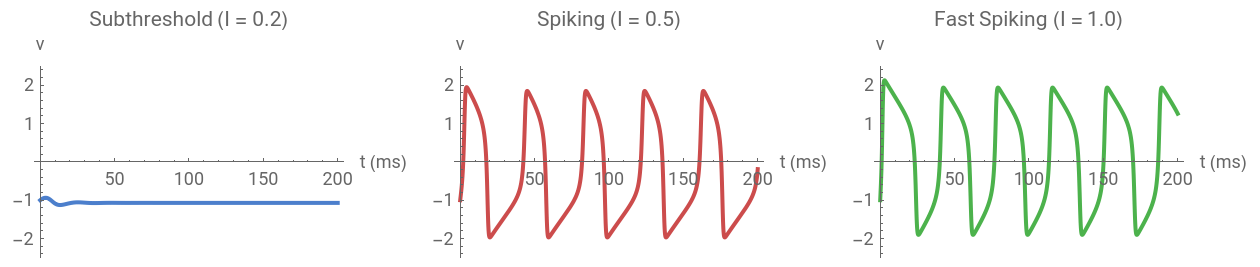
Let’s first just watch a neuron respond to different input currents. Below threshold signals silence and above threshold signals repetitive spiking. This is the fundamental principle of neural computation.
Out[]=
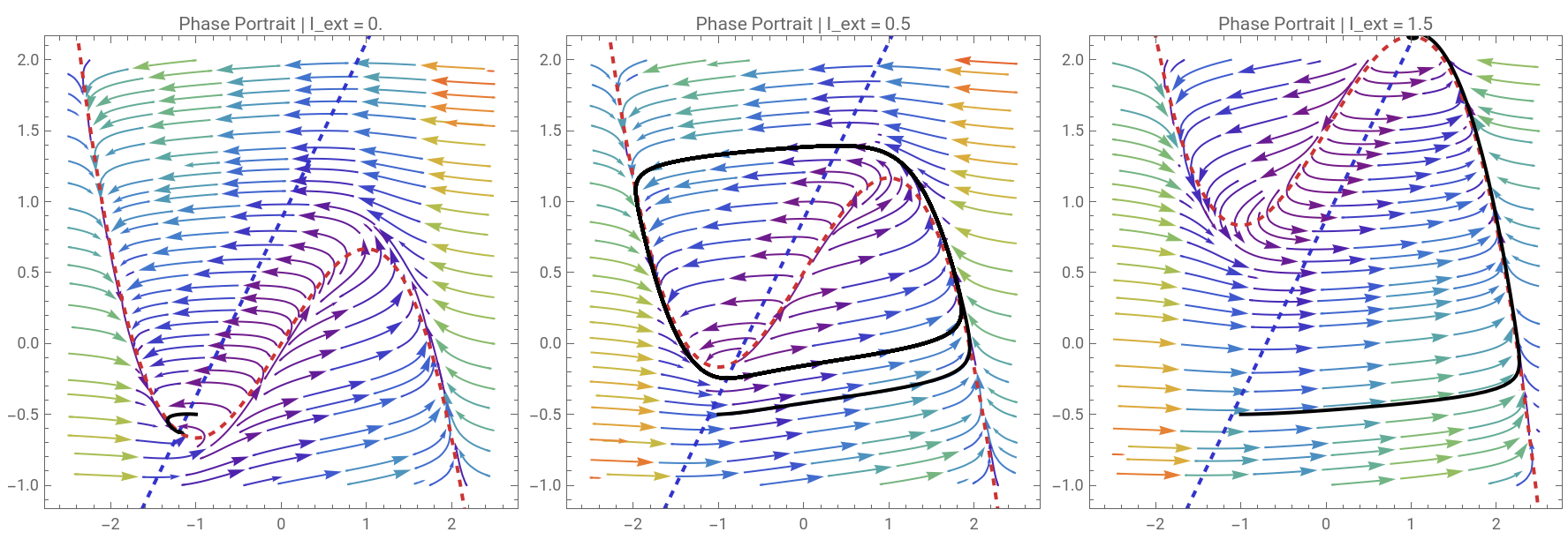
The phase portrait is where the FHN model really shines. The v-nullcline (cubic) and w-nullcline (linear) partition the phase plane. Their intersection determines the fixed point, and the relative position determines whether the system rests, oscillates, or is excitable.
Out[]=
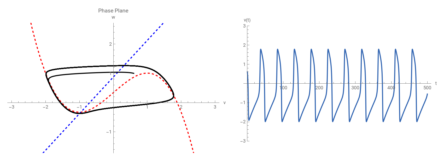
We can also demonstrate how each parameter reshapes the dynamics. The moment the fixed point destabilizes is the Hopf bifurcation, and it’s the mathematical origin of neural spiking.
Manipulate[Module[{sol,vNull,wNull,traj,timeSeries},sol=Quiet@NDSolve[{v'[t]==v[t]-v[t]^3/3-w[t]+Iext,w'[t]==eps*(v[t]+0.7-0.8*w[t]),v[0]==v0,w[0]==w0},{v,w},{t,0,tMax},MaxSteps->50000];vNull=Plot[x-x^3/3+Iext,{x,-3,3},PlotStyle->{Thick,Red,Dashed}];wNull=Plot[(x+0.7)/0.8,{x,-3,3},PlotStyle->{Thick,Blue,Dashed}];traj=ParametricPlot[Evaluate[{v[t],w[t]}/.sol],{t,0,tMax},PlotStyle->{Thick,Black}];timeSeries=Plot[Evaluate[v[t]/.sol],{t,0,tMax},PlotStyle->{Thick,RGBColor[0.2,0.4,0.7]},AxesLabel->{"t","v(t)"},PlotRange->{-3,3}];GraphicsRow[{Show[vNull,wNull,traj,PlotRange->{{-3,3},{-1.5,2.5}},AxesLabel->{"v","w"},PlotLabel->"Phase Plane",ImageSize->400],timeSeries},ImageSize->850]],Style["External Current",Bold],{{Iext,0.34,"I_ext"},-0.5,2.0,0.01},Delimiter,Style["Model Parameters",Bold],{{eps,0.08,"ϵ"},0.01,0.5,0.01},Delimiter,Style["Initial Conditions",Bold],{{v0,-1.0,"v(0)"},-2.5,2.5,0.1},{{w0,-0.5,"w(0)"},-1.5,2.0,0.1},{{tMax,200,"t_max"},50,500,10},ControlPlacement->Left,TrackedSymbols:>{Iext,eps,v0,w0,tMax},SaveDefinitions->True]
Out[]=


Bifurcation Analysis: How Neurons Switch Regimes
Bifurcation Analysis: How Neurons Switch Regimes
The most important question in computational neuroscience is what makes a neuron start firing? The answer is a Hopf bifurcation, which is a qualitative change in dynamics as the input current crosses a critical threshold. Different bifurcation types produce different computational properties. Type I neurons can fire at arbitrarily low rates (good for rate coding), and Type II neurons have a minimum frequency (good for synchronization).
Out[]=
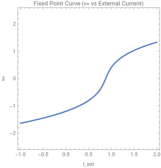
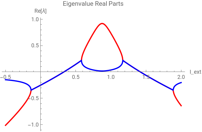
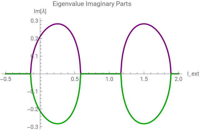
We linearize around the fixed point and track the eigenvalues. When the real part crosses zero, we get a Hopf bifurcation. The imaginary part at the crossing gives the initial oscillation frequency, i.e., the neuron’s preferred firing rate.
Out[]=




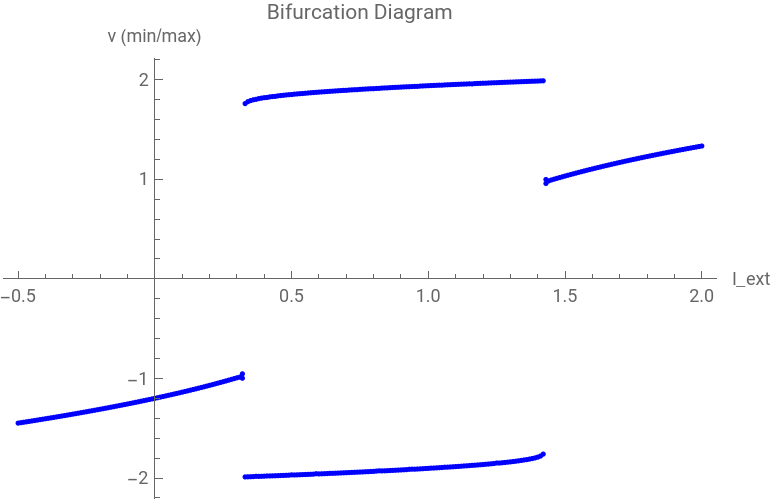
For each value of I_ext, we run the system to steady state and record the min and max of v(t). Below the bifurcation, a single dot means resting and above two dots means spike peaks and troughs that separate as current increases.
Out[]=
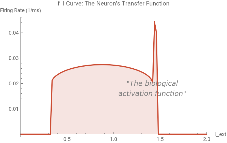
In neuroscience, the f-I curve characterizes a neuron’s transfer function, the mapping from input to output firing rate. This is essentially the neuron’s activation function. Keep this in mind for Part 4.
Out[]=
Coupled Networks & Biological Sparsity
Coupled Networks & Biological Sparsity
Real brains have ~86 billion neurons, but at any moment only about are active. Sparse representations are energy-efficient, high-capacity, and robust to noise. Let’s build a small network and see how sparsity emerges naturally from FHN excitability.
We give each neuron a different (heterogeneous) baseline current: some near threshold, some below, some above. The coupling allows active neurons to recruit silent ones. In the raster plot below, each row is a neuron and each dot is a spike.
Now let’s quantify sparsity. We’ll measure:
• Lifetime sparsity: for each neuron, what fraction of time is it active?
• Population sparsity: at each time point, what fraction of neurons are active?
• Kurtosis: how heavy-tailed is the activity distribution? (Higher = sparser)
• Lifetime sparsity: for each neuron, what fraction of time is it active?
• Population sparsity: at each time point, what fraction of neurons are active?
• Kurtosis: how heavy-tailed is the activity distribution? (Higher = sparser)
What happens to sparsity as we change connection density? Too sparse a network isolated neurons. Too dense synchronized epileptic-like activity. Biology operates in the sweet spot.
The AI Bridge: From Neurons to Deep Learning
The AI Bridge: From Neurons to Deep Learning
The principles we’ve been studying in biological neurons (thresholded excitability, sparse activation, and nonlinear transfer functions) are exactly the same principles powering modern artificial neural networks. The convergence isn’t coincidence. It reflects deep mathematical truths about efficient information processing.
Remember the f-I curve from Part 2? That’s the neuron’s input-output relationship. Compare it to the activation functions used in AI.
In both biological and artificial networks, sparsity means most units are inactive (zero output) at any given time. Let’s simulate a simple artificial network layer and compare its activation statistics to our FHN network.
Conclusion and Future Directions
Conclusion and Future Directions
This project used the FitzHugh-Nagumo model to describe single-neuron dynamics all the way to the design principles of modern AI. By analyzing how a neuron’s equations produce threshold behavior, we showed that firing onset is a natural consequence of the system’s geometry rather than a special rule built in by hand. Extending to small networks of neurons with varied excitability showed that sparse activity emerges automatically at the right level of connectivity, matching what we observe in real brains. Future work could incorporate inhibitory neurons to study how they regulate sparsity, add a learning rule to connect these dynamics to memory formation, and test whether the model’s activity statistics hold up against real electrophysiology data.
References
References
◼
FitzHugh, Richard. “Impulses and physiological states in theoretical models of nerve membrane.” Biophysical journal 1.6 (1961): 445-466. DOI: https://doi.org/10.1016/S0006-3495(61)86902-6
◼
Hodgkin, Alan L., and Andrew F. Huxley. “A quantitative description of membrane current and its application to conduction and excitation in nerve.” The Journal of physiology 117.4 (1952): 500. DOI: https://doi.org/10.1113/jphysiol.1952.sp004764
◼
Izhikevich, Eugene M. Dynamical systems in neuroscience. MIT press, 2007.
◼
Olshausen, Bruno A., and David J. Field. “Emergence of simple-cell receptive field properties by learning a sparse code for natural images.” Nature 381.6583 (1996): 607-609. DOI: https://doi.org/10.1038/381607a0
◼
Lillicrap, Timothy P., et al. “Backpropagation and the brain.” Nature Reviews Neuroscience 21.6 (2020): 335-346. DOI: https://doi.org/10.1038/s41583-020-0277-3
CITE THIS NOTEBOOK
CITE THIS NOTEBOOK
Bridging biological neurons and AI: excitability, Hopf bifurcations, and sparsity in FHN
by Guhan Thiagarajan
Wolfram Community, STAFF PICKS, April 6, 2026
https://community.wolfram.com/groups/-/m/t/3674654
by Guhan Thiagarajan
Wolfram Community, STAFF PICKS, April 6, 2026
https://community.wolfram.com/groups/-/m/t/3674654