FontenéSecondTheorem::usage="Fontené's second theorem states that if a point moves on a straight line what passes through the circumcenter, then its pedal circle passes through a fixed point on the circle of the 9 points. References: Wolfram MathWorld: Fontené theorems, Pedal circle, Pedal triangle; Personal."
Example 1:
In[]:=
Manipulatex1=-2;y1=5;x2=7;y2=12;x3=9;y3=-4;tri={{-2,5},{7,12},{9,-4}};α=TriangleCenter[tri,"Circumcenter"];α1=TriangleMeasurement[tri,"Circumradius"];xc=α[[1]];yc=α[[2]];Circumcenter={xc,yc};β=TriangleCenter[tri,"NinePointCenter"];xn=β[[1]];yn=β[[2]];β1=TriangleMeasurement[tri,"NinePointRadius"];P={x,yc+x-xc};PN=,;PP1=-,-+;PP2=,-;PP3=-+,+;tri1={PP1,PP2,PP3};ξ=TriangleCenter[tri1,"Circumcenter"];xc1=ξ[[1]];yc1=ξ[[2]];ξ1=TriangleMeasurement[tri1,"Circumradius"];Show[{ContourPlot[x-y-xc+yc==0,{x,-15,15},{y,-15,15},ContourStyle->{Black,Thick}],Graphics[{Red,Line[{P,PP1}]}]/.xk1,Graphics[{Red,Line[{P,PP2}]}]/.xk1,Graphics[{Red,Line[{P,PP3}]}]/.xk1,Graphics[{Blue,Dashed,InfiniteLine[{{x1,y1},{x2,y2}}]}],Graphics[{Blue,Dashed,InfiniteLine[{{x1,y1},{x3,y3}}]}],Graphics[{Blue,Dashed,InfiniteLine[{{x2,y2},{x3,y3}}]}],Graphics[{DarkGreen,TriangleConstruct[tri1,"Boundary"]}]/.xk1,Graphics[{Black,PointSize[0.01],Point[P],Text[Style["P",14,Bold],P,{0,-1.2}]}]/.xk1,Graphics[{Black,Dashed,Circle[{xn,yn},β1]}],Graphics[{Green,PointSize[0.01],Point[Circumcenter],Text[Style["C",14,Bold],Circumcenter,{0,-1.2}]}],Graphics[{Blue,PointSize[0.01],Point[{x1,y1}],Text[Style["",14,Bold],{x1,y1},{0,-1.2}]}],Graphics[{Blue,PointSize[0.01],Point[{x2,y2}],Text[Style["",14,Bold],{x2,y2},{0,-1.2}]}],Graphics[{Blue,PointSize[0.01],Point[{x3,y3}],Text[Style["",14,Bold],{x3,y3},{0,-1.2}]}],Graphics[{Red,PointSize[0.01],Point[PP1]}]/.xk1,Graphics[{Red,PointSize[0.01],Point[PP2]}]/.xk1,Graphics[{Red,PointSize[0.01],Point[PP3]}]/.xk1,Graphics[{Purple,Circle[{xc1,yc1},ξ1]}]/.xk1,Graphics[{Blue,TriangleConstruct[tri,"Boundary"]}],Graphics[{Brown,PointSize[0.01],Point[PN],Text[Style["F",14,Bold],PN,{0,-1.2}]}]},AxesTrue,AxesLabel{x,y},AxesOrigin{0,0},AspectRatioAutomatic,PlotRange15,ImageSize700],{k1,-15,15,0.00001},ContinuousAction->True
683
158
1
2
44496
5135
7x
65
6788
5135
56x
65
45117+1738x
15958
16763
15958
9x
101
44597
10270
72x
65
32639
10270
56x
65
P
2
P
2
P
3
Out[]=


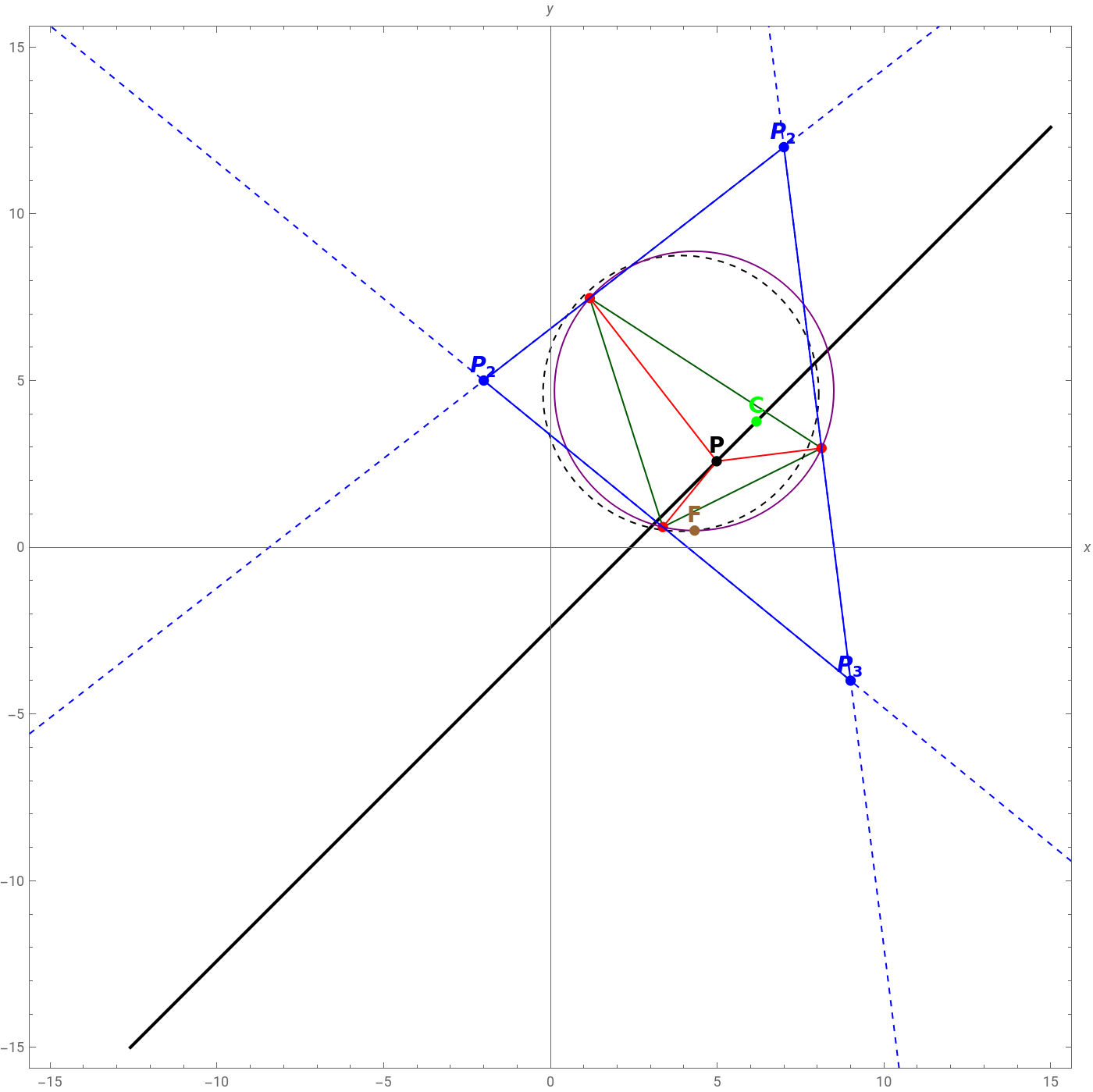
In the animation the theorem is checked. The pedal circumference always passes through the point F, of the circumference of the 9 points.
Example 2:
In[]:=
Manipulate[x1=0;y1=0;x2=1;y2=0;x3=0.3;y3=0.7;tri={{0,0},{1,0},{.3,.7}};α=TriangleCenter[tri,"Circumcenter"];α1=TriangleMeasurement[tri,"Circumradius"];xc=α[[1]];yc=α[[2]];Circumcenter={xc,yc};β=TriangleCenter[tri,"NinePointCenter"];xn=β[[1]];yn=β[[2]];β1=TriangleMeasurement[tri,"NinePointRadius"];P={x,yc+0.5(x-xc)};PN={0.5399999999989418`,0.48000000000064413`};PP1={0.5250000000000002`+0.24999999999999983`x,0.47500000000000014`-0.2500000000000003`x};PP2={-0.01810344827586198`+0.33620689655172403`x,-0.04224137931034465`+0.7844827586206894`x};PP3={1.`x,0};tri1={PP1,PP2,PP3};ξ=TriangleCenter[tri1,"Circumcenter"];xc1=ξ[[1]];yc1=ξ[[2]];ξ1=TriangleMeasurement[tri1,"Circumradius"];Show[{ContourPlot[0.5x-y-0.5xc+yc==0,{x,-2,2},{y,-2,2},ContourStyle->{Black,Thick}],Graphics[{Red,Line[{P,PP1}]}]/.xk1,Graphics[{Red,Line[{P,PP2}]}]/.xk1,Graphics[{Red,Line[{P,PP3}]}]/.xk1,Graphics[{Blue,Dashed,InfiniteLine[{{x1,y1},{x2,y2}}]}],Graphics[{Blue,Dashed,InfiniteLine[{{x1,y1},{x3,y3}}]}],Graphics[{Blue,Dashed,InfiniteLine[{{x2,y2},{x3,y3}}]}],Graphics[{DarkGreen,TriangleConstruct[tri1,"Boundary"]}]/.xk1,Graphics[{Black,PointSize[0.01],Point[P],Text[Style["P",14,Bold],P,{0,-1.2}]}]/.xk1,Graphics[{Black,Dashed,Circle[{xn,yn},β1]}],Graphics[{Green,PointSize[0.01],Point[Circumcenter],Text[Style["C",14,Bold],Circumcenter,{0,-1.2}]}],Graphics[{Blue,PointSize[0.01],Point[{x1,y1}],Text[Style["",14,Bold],{x1,y1},{0,-1.2}]}],Graphics[{Blue,PointSize[0.01],Point[{x2,y2}],Text[Style["",14,Bold],{x2,y2},{0,-1.2}]}],Graphics[{Blue,PointSize[0.01],Point[{x3,y3}],Text[Style["",14,Bold],{x3,y3},{0,-1.2}]}],Graphics[{Red,PointSize[0.01],Point[PP1]}]/.xk1,Graphics[{Red,PointSize[0.01],Point[PP2]}]/.xk1,Graphics[{Red,PointSize[0.01],Point[PP3]}]/.xk1,Graphics[{Purple,Circle[{xc1,yc1},Abs[ξ1]]}]/.xk1,Graphics[{Blue,TriangleConstruct[tri,"Boundary"]}],Graphics[{Brown,PointSize[0.01],Point[PN],Text[Style["F",14,Bold],PN,{0,-1.2}]}]},AxesTrue,AxesLabel{x,y},AxesOrigin{0,0},AspectRatioAutomatic,PlotRange2,ImageSize700],{k1,-2,2,0.00001},ContinuousAction->True]
P
2
P
2
P
3
Out[]=
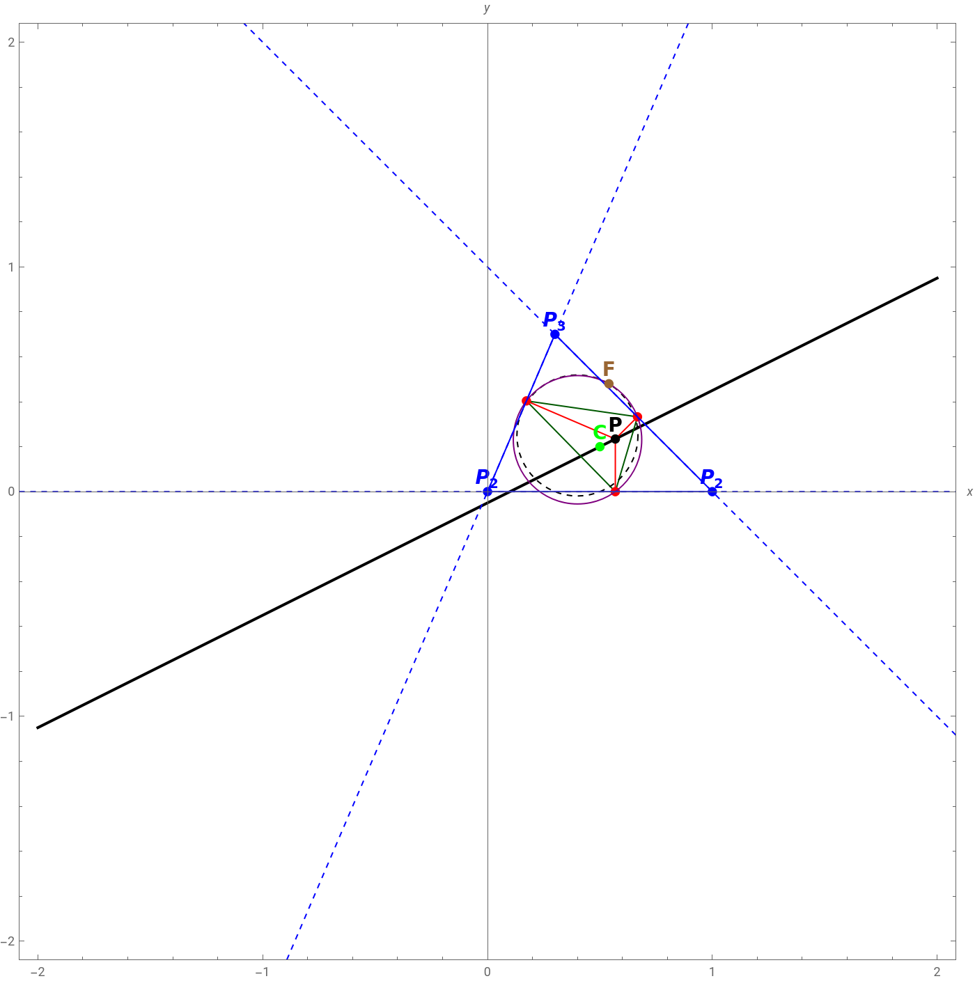
In the animation the theorem is checked. The pedal circumference always passes through the point F, of the circumference of the 9 points.