The optimization of the thrust-to-power ratio in ion propulsion systems presents a significant challenge in advancing space propulsion technologies. This study focuses on developing rough models and simulation frameworks on both Gridded Ion Thrusters and Hall Effect thrusters to address this issue. My findings indicate that the integration of advanced computational techniques significantly enhances the understanding of ion propulsion mechanisms and provides a rough simulation model for future advancements in space propulsion technology. These results contribute to the development of more efficient and reliable ion engines, which are essential for long-duration space missions and interplanetary exploration.
Introduction
Introduction
In my research, I define the physical parameters of the two ion engines, like the charge densities of the anode and cathode, magnetic field strengths, as well as the radius and lengths of the thrusters. I use these parameters to calculate the electric and magnetic field distributions and ionization processes, and use Mathematica’ s differential equation solvers to simulate ion motion. Through these simulations, I identify the optimal operating parameters that maximize the thrust-to-power ratio. Extensive parameter sweeps and sensitivity analyses are conducted to examine the effects of various input variables on engine performance. I then compared my results to empirical data the U of Michigan PEPL lab have gathered through experimentation and published onto a Julia Package to verify the accuracy of my simulation.
Gridded Ion Thruster
Gridded Ion Thruster
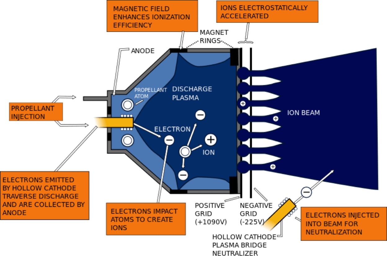
A Gridded Ion Thruster utilizes electrostatic magnetic fields to accelerate the ions to produce thrust. Typically, Hall Thrusters consists of mainly an anode shell, a positively charged screening grid, and a negatively charge accelerating grid. electron guns are placed inside the anode shell to ionize the propellant within the anode shell and outside the thruster to neutralize the resulting ions. Once the propellant is ionized, the electrostatic forces generated by the anode push the ion towards the screening and acceleration grids. Since the grids are so close to each other and oppositely charged, a massive electric field is generated which accelerates the ions up to eighty kilometers per second.
In[]:=
Calibrating the Gridded Ion Thruster Simulation
Calibrating the Gridded Ion Thruster Simulation
Defining the Gridded Ion Thruster Regions
Defining the Gridded Ion Thruster Regions
First we define the initial conditions for the anode and grids of the gridded ion thruster.
In[]:=
anodeOuterRadius=0.4;anodeThickness=0.04;anodeInnerRadius=anodeOuterRadius-anodeThickness;anodeHeight=0.45; baseHeight=anodeThickness;gridSpacing=0.035;gridRadius=anodeOuterRadius;gridHeight=0.006;
We now define the domain for the calculation of the electric potential.
In[]:=
domain[anodeOuterRadius_,anodeHeight_]:= ImplicitRegion[(-0.5 + (-1.25*anodeOuterRadius)) <= x <= (0.5 + (1.25*anodeOuterRadius)) && (-0.5 + (-1.25*anodeOuterRadius)) <= y <= (0.5 + (1.25*anodeOuterRadius)) && Min[-0.5, -(2*anodeHeight)] <= z <= Max[1, 3*anodeHeight], {x, y, z}];
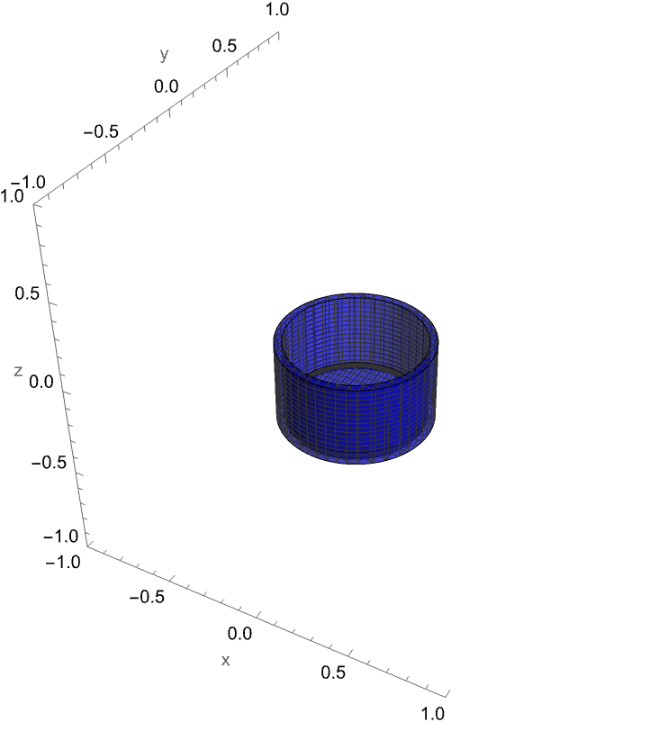
We can proceed to create the shape for the anode region which includes the walls and base plate of the anode.
In[]:=
anode[anodeInnerRadius_,anodeOuterRadius_,anodeHeight_]:=ImplicitRegion[(anodeInnerRadius^2<=x^2+y^2<=anodeOuterRadius^2)&&(-anodeHeight<=z<=0),{x,y,z}];base[anodeOuterRadius_,anodeThickness_,anodeHeight_]:=ImplicitRegion[x^2+y^2<=(anodeOuterRadius-anodeThickness)^2&&-anodeHeight<=z<=-anodeHeight+anodeThickness,{x,y,z}];
Now lets visualize the anode regions.
In[]:=
anodePlot=RegionPlot3D[(anodeInnerRadius^2<=x^2+y^2<=anodeOuterRadius^2)&&(-anodeHeight<=z<=0),{x,-anodeOuterRadius,anodeOuterRadius},{y,-anodeOuterRadius,anodeOuterRadius},{z,-anodeHeight,0},PlotRange->{{-1,1},{-1,1},{-1,1}},PlotPoints->100,MaxRecursion->2,Boxed->False,Axes->True,AxesLabel->{"x","y","z"},PlotStyle->Directive[Opacity[0.5],Blue]];basePlot=RegionPlot3D[(x^2+y^2<=(anodeOuterRadius-anodeThickness)^2)&&(-anodeHeight<=z<=-anodeHeight+anodeOuterRadius-anodeInnerRadius),{x,-anodeOuterRadius,anodeOuterRadius},{y,-anodeOuterRadius,anodeOuterRadius},{z,-anodeHeight,-anodeHeight+anodeThickness},PlotRange->{{-1,1},{-1,1},{-1,1}},PlotPoints->30,MaxRecursion->2,Boxed->False,Axes->True,AxesLabel->{"x","y","z"},PlotStyle->Directive[Opacity[0.5],Blue]];Show[anodePlot,basePlot]
Out[]=
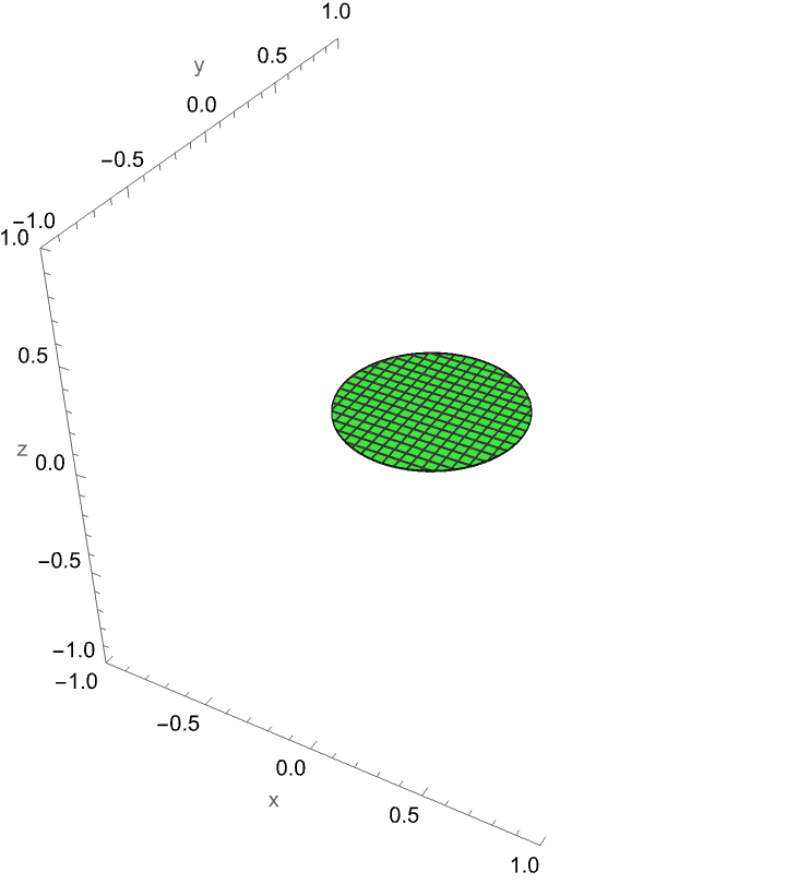
Define and visualize the positively charged screening grid region.
In[]:=
firstGrid[gridRadius_,gridHeight_]:=ImplicitRegion[x^2+y^2<=gridRadius^2&&0.01<=z<=(0.01+gridHeight),{x,y,z}];
In[]:=
firstGridPlot=RegionPlot3D[x^2+y^2<=gridRadius^2&&0.01<=z<=(0.01+gridHeight),{x,-gridRadius,gridRadius},{y,-gridRadius,gridRadius},{z,0.01,0.01+gridHeight},PlotRange->{{-1,1},{-1,1},{-1,1}},PlotPoints->20,MaxRecursion->2,Boxed->False,Axes->True,AxesLabel->{"x","y","z"},PlotStyle->Directive[Opacity[0.5],Green]]
Out[]=
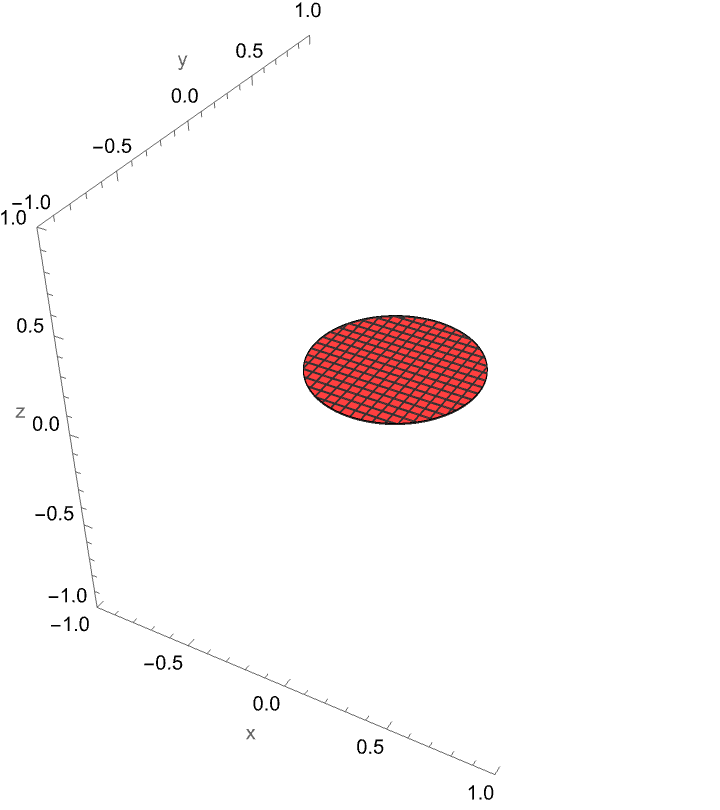
Create and visualize the second negatively charged acceleration grid.
In[]:=
secondGrid[gridRadius_,gridSpacing_,gridHeight_]:=ImplicitRegion[x^2+y^2<=gridRadius^2&&(0.01+gridSpacing+gridHeight)<=z<=(0.01+gridSpacing)+2*gridHeight,{x,y,z}];
In[]:=
secondGridPlot=RegionPlot3D[x^2+y^2<=gridRadius^2&&(0.01+gridSpacing+gridHeight)<=z<=(0.01+gridSpacing)+2*gridHeight,{x,-gridRadius,gridRadius},{y,-gridRadius,gridRadius},{z,(0.01+gridSpacing+gridHeight),(0.01+gridSpacing)+2*gridHeight},PlotRange->{{-1,1},{-1,1},{-1,1}},PlotPoints->30,MaxRecursion->2,Boxed->False,Axes->True,AxesLabel->{"x","y","z"},PlotStyle->Directive[Opacity[0.5],Red]]
Out[]=
This is how everything looks together.
Generating the Electrostatic Field
Generating the Electrostatic Field
Setup Poisson’s equation for our situation by assigning the charge densities for each region and taking the Laplace Operator for the regions.
We specify the boundary conditions at the outer boundary of the domain:
And finally, solve the partial differential equation to get the electrostatic potential at each point:
Visualize the electric potential and how the current structure of the thruster affects the forces
Calculating the Trajectory of the Ion
Calculating the Trajectory of the Ion
Now that all of our regions and forces are setup, we must now calculate the trajectory of the ion in order to see its velocity and acceleration.
Most ion thrusters use Xenon, thus we have to define its properties for simulation.
We need to convert the electric potential to a gradient.
Define the equations of motion.
Calculate the trajectory of the ion.
Extract the ion’s trajectory.
Visualizing the trajectory plot with the electric potential and ion thruster plots we can how the ion travels in relation to the thruster.
Trajectory and Thrust Analysis
Trajectory and Thrust Analysis
Calculate and plot the velocity in the Z direction against time.
Calculate and plot the acceleration in the Z direction against time.
Plotting the acceleration and velocity against the z coordinate could provide a clearer visualization.
Generate the time points
Evaluate the z - coordinates, velocity, and acceleration at the time points
Plot the velocity against the z coordinate.
Plot the acceleration against the z coordinate.
From the acceleration plot, we can confirm that our thruster mimics the physics of a real gridded ion thruster accurately as there is a spike in acceleration between the screening and acceleration grid which occurs due to the large electrostatic potential between the two grids.
Extract the maximum velocity of the ion.
Calculate the mass flow rate and the total thrust generated from the thruster in milliNewtons.
Calculate the power consumption in Watts based on the amount of energy it would take to accelerate the ions to their speeds.
Calculate the thrust to power ratio.
Optimization of the Gridded Ion Thruster
Optimization of the Gridded Ion Thruster
The gridded ion thruster can range immensely in sizes, and these parameters can drastically affect the thrust and power consumption of the thruster. The parameters we will try to optimize will be the anode radius, anode thickness, anode height, grid spacing, and grid height.
Running the Optimization Simulations
Running the Optimization Simulations
After setting up the simulation, we can now combine all the relevant functions into one function to be used for optimization.
Here are the Plausible ranges for each parameter in meters:
Run the simulation for all plausible parameters.
Analyzing the Optimization Results
Analyzing the Optimization Results
Define the labels for each item in the output.
Separate each item in the results.
Convert the results into a matrix
Create a correlation heat map between the different parameters and results to clearly visualize their relationships.
From the correlation heat map, we can see that there is a positive correlation between thrust and many of the parameters, but the correlation between the thrust-to-power ratio and the parameters is much weaker or even negative. Therefore to maximize thrust, we could simply infinitely scale up the entire thruster, but that would require an unattainable amount of input power. Therefore a balance between the thruster size and input power must be found. This balance can be found by maximizing the thrust-to-power ratio.
Find the parameters that maximize thrust.
Find the parameters that maximize the thrust-to-weight ratio.
Theoretically by using these parameters for a gridded ion engine, one could generate around 26 milliNewtons of thrust while only consuming around 360 Watts of power, which is much cheaper than the 1000 Watts typically needed to generate the same amount of thrust.
Hall Thruster
Hall Thruster
A Hall Thruster is different from a Gridded Ion Thruster in which it is a coaxial device where orthogonal electric and magnetic fields are used to ionize the propellant and accelerate the resulting ions to produce thrust. Typically, Hall Thrusters consists of multiple parts, the anode, the cathode, and surrounding magnets. A cathode neutralizer is placed either around the thruster or in the middle which shoots electrons to be used by the thruster to ionize the propellant and neutralize the resulting ions. Magnets are placed around the annulus to create a a radial magnetic field that traps electrons in the annulus. The electrons spin around in the annulus in which they are used to ionize the propellant. An anode shell is used to inject the propellant into the annulus where the propellant atoms are ionized by the constantly rotating electrons. Once the propellant is ionized, the electrostatic forces generated by the anode and cathode as well as the Lorenz force caused by the electric field accelerate the ion to tremendous speeds up to fifty kilometers per second.
Calibrating the Hall thruster Simulation
Calibrating the Hall thruster Simulation
Defining the Hall Thruster’s Regions
Defining the Hall Thruster’s Regions
I decided to simulate the design in which the anode is placed in the middle of the thruster instead of on the edges.
First we must define the initial Parameters for the thruster.
Define the cathode region.
Visualize the cathode region.
Define the anode region, which can be split into the anode walls and base.
Visualize the anode region.
Even though the plasma is not used in the simulation, it is still useful to visualize the plasma region as this is where the electron clouds will be traveling.
Visualize the plasma region.
In a Hall Thruster, the magnets in the inner and outer regions must be reversed to ensure there is a radial magnetic field running from the inner magnets to the outer magnets.
Define the north and south regions of the inner magnet.
Visualize the inner magnet.
Define the north and south regions of the outer magnet.
Visualize the outer magnet.
Now we can combine all the plots to visualize the entire hall thruster.
Generating the Electrostatic Field
Generating the Electrostatic Field
First, let’s define the charge density of the anode and cathode as well as the domain for the electrostatic field.
Next we can setup Poisson’s equation and the boundary conditions for our simulation.
Solve the partial differential equation to get the electrostatic potential at each point.
Visualize the electrostatic Field.
Generating the Magnetic Field
Generating the Magnetic Field
In a hall thruster, the inner and outer magnets must be oriented oppositely to ensure the magnetic field properly flows radially from the inner to the outer magnets to trap the electrons in the annulus.
First let’s define the base strengths of the magnets and the magnetic permeability of a vacuum, which is where the thruster will most likely be running.
Now, we must further refine the strength of each magnetic region
The magnetic field generated by a constant current flow is defined by the biot Savart Law:
Set up the function to use the Biot Savart Law to solve for the magnetic field.
Define the function to calculate the inner and outer magnet’s magnetic fields.
Combine all the functions to create one magnetic field that utilizes all the magnet’s regions.
Visualize the magnetic and electric Field.
Calculating the Trajectory of the Ion
Calculating the Trajectory of the Ion
Now that all of our regions and forces are setup, we must now calculate the trajectory of the ion in order to see its velocity and acceleration.
First we must define the initial positions and properties for Xenon.
Convert the electric field to a gradient.
Similarly to the gridded ion thruster, we must create the equation of motions but we must take both the electrostatic field forces and the magnetic field forces into account.
Solve the equations of motion to find the trajectory of the ion.
Plot the trajectory of the ion.
Trajectory and Thrust Analysis
Trajectory and Thrust Analysis
Find the exhaust velocity of the ion.
Find and plot the acceleration of the ion.
Generate the time points.
Plotting the acceleration and velocity against the z coordinate could provide a clearer visualization.
Evaluate the z-coordinates, velocity, and acceleration at the time points.
Plot the velocity against the z coordinate.
Plot the acceleration against the z coordinate.
Mass flow rate:
Calculate the power usage in Watts.
Finally, we can calculate the thrust-to-power ratio.
Comparing My Data To Real Simulations
Comparing My Data To Real Simulations
I found a Julia Package from the University of Michigan‘s Plasmadynamics and Electric Propulsion Laboratory that had gathered data on a real Hall Thruster and had published it. I can use their data to compare it to my simulation to ensure my simulation has an anchor to reality. In their simulation, they collected their data along the horizontal dimension of the annulus, which they stated to be eight centimeters deep.
Importing and Processing the Data
Importing and Processing the Data
Let’s first import the necessary data:
The data is initially plotted against time, which isn’t great for visualization, therefore we must convert the time coordinates to the corresponding distance coordinates.
Plotting the data
Plotting the data
Let’s plot all the data to get a clear visualization of their values.
Comparing the Simulations
Comparing the Simulations
Now that we have data from both my simulation and that from the Julia Notebook, we can compare our results to see how accurate my simulation is. Since their annulus had a depth of eight centimeters, we must ensure our simulation’s parameters create an annulus depth of the same length. We must also ensure the thruster area used to calculate the thrust on both is the same.
First let’s define the conditions needed to calculate the thrust for the Julia Package.
Next, we have to calculate the relevant variables needed to calculate thrust like the mass flow rate and the exhaust velocity.
We must also make the necessary calculations needed to solve for the power consumption.
Let’s compare the velocity plots of both thrusters.
We can also compare the exhaust velocity of the ions.
Based on the velocity plots and the values, we can see that my simulation has a slightly greater exhaust velocity, but the Julia Package data ends right where the ion leaves the thruster, but typically the ion continues to accelerate for a while longer which the package does not capture, and the velocity values are very similar already.
Due to my simulation’s higher exhaust velocity, it makes sense that the thrust generated is higher.
Based on these comparisons, it seems that our simulation is relatively accurate and we can proceed with the optimization.
Optimization of the Hall Thruster
Optimization of the Hall Thruster
Much like the gridded ion thruster, the Hall Thruster can range immensely in sizes, and these parameters can also drastically affect the thrust and power consumption of the thruster. The parameters we will try to optimize will be the anode radius, anode thickness, anode length, cathode radius, and inner magnet radius.
Running the Optimization Simulations
Running the Optimization Simulations
After setting up the simulation, we can now combine all the relevant functions into one function to be used for optimization .
Plausible ranges for each parameter in meters:
Run the simulation for all plausible parameters.
Analyzing the Optimization Results
Analyzing the Optimization Results
Define the labels for each item in the output.
Separate each item in the results.
Convert the data into a matrix
Create a correlation heat map between the different parameters and results to clearly visualize their relationships.
From the correlation heat map, we can once again see that there is a positive correlation between thrust and many of the parameters, but the correlation between the thrust-to-power ratio and the parameters is much weaker or even negative, much more so than for the gridded ion thruster. Therefore to maximize the thrust-to-power ratio, we must ensure to balance between the anode radius which strongly correlates positively with thrust while ensuring the anode thickness and length are not too long as they strongly correlate negatively with the thrust-to-power ratio.
Find the parameters to maximize thrust.
Find the parameters to maximize the thrust-to-power ratio.
From these results we can see that by maximizing the thrust-to-weight ratio we would theoretically be able to achieve 185 miliNewtons of thrust while consuming less than 1967 Watts of power. The typical Hall thruster operates at around 1350 Watts and produces 83 mN of thrust, but based on our simulation we would be able to increase the thrust by 2.22 times while only increasing the power consumption by 1.456 times.
Conclusion
Conclusion
In this research project, we explored the forces that create thrust in gridded ion and hall effect thrusters. Using existing data on hall thrusters, we ensured that our simulations had a high degree of accuracy and that our data can be applied to the real world. The correlation heat maps identified the relationships between different parameters on the thrust-to-power ratio and showed that there must be a careful balance between each parameter in order to achieve a high thrust-to-power ratio. Overall, this project contributed to the understanding of how different parameters affect the within the thruster used to accelerate the ions and provided a foundation for future research in this area.
Limitations and Future Directions
Limitations and Future Directions
Due to the inherent complexity in this topic, it is very difficult to make a fully accurate simulation without access to a real ion thruster for me to actively compare my data to. My simulation is also a simplification of the real process as I did not take the friction of the plasma into account nor did I simulate the ionization process of the propellant. Some future work I could conduct would be to convert the Julia Package I used to Mathematica so I could more effectively run their simulation and conduct data analysis on it. I could also do 2D simulations that take the ionization process and friction into account for a easier more accurate simulation.
Acknowledgments
Acknowledgments
I would like to thank my mentor Shenghui Yang deeply for supporting me and guiding me throughout my research as well as the WSRP program for allowing me this opportunity to pursue my interests. I would also like to thank Nicolo Monti for supporting me along my process.
Works Cited
Works Cited
◼
Chow TT, Miskimin CR, Roeder PT. Application of Field Emission Cathode Technology to Ion Thrusters. IEPC. 1985. https://electricrocket.org/IEPC/85_2.pdf
◼
“Hall Thruster.” ScienceDirect Topics, Elsevier. https://www.sciencedirect.com/topics/engineering/hall-thruster
◼
Hofer RR. Development and Characterization of High-Efficiency, High-Specific Impulse Xenon Thrusters. AIAA. 2023. https://arc.aiaa.org/doi/pdf/10.2514/6.2023-71410
◼
Brophy J, Polk J, Rawlin V. Ion Thruster Development. IEPC. 1993. https://electricrocket.org/IEPC/IEPC1993-066.pdf
◼
Gallimore A, Goebel D, Hofer R. Development of Ion and Hall Thrusters. AIAA. 1996. https://pepl.engin.umich.edu/pdf/AIAA-96-2973.pdf
◼
Boyd I, Dressler R. Ion Thruster Modeling: Particle Simulations and Experimental Validations. Journal of Propulsion and Power. 2002. https://www.researchgate.net/publication/234894818_Ion_Thruster_Modeling_Particle_Simulations_and_Experimental_Validations
◼
Spores R, Spores E. Short Review on Electric Propulsion System: Ion Thruster. Journal of Propulsion and Power. 2014. https://www.researchgate.net/publication/264977125_Short_Review_on_Electric_Propulsion_System_Ion_Thruster
◼
Marks T, Schedler P, Jorns B. HallThruster.jl: A Julia Package for 1D Hall Thruster Discharge Simulation. Journal of Open Source Software. 2023. https://joss.theoj.org/papers/10.21105/joss.04672
◼
Goebel D, Katz I. Ion and Hall Thruster Grid Technology. JPL Technical Report. 2008.
descanso.jpl.nasa.gov/SciTechBook/series1/Goebel_05_Chap5_Grids.pdf.
descanso.jpl.nasa.gov/SciTechBook/series1/Goebel_05_Chap5_Grids.pdf.
◼
Goebel D, Katz I. Fundamentals of Electric Propulsion: Ion and Hall Thrusters. JPL Technical Report. 2008. https://descanso.jpl.nasa.gov/SciTechBook/series1/Goebel__cmprsd_opt.pdf
◼
Morozov A. Hall Thruster Geometry. Journal of Applied Physics. 2000. https://www.researchgate.net/publication/337085936_Thomson_scattering_investigations_of_a_low-power_Hall_thruster_in_standard_and_magnetically-shielded_configurations
◼
“Biot-Savart Law.” Byju’s. https://byjus.com/physics/biot-savart-law/
◼
Heuveline V. Lectures on Mathematical Methods for Physicists. University of Cambridge. 2005. https://www.damtp.cam.ac.uk/user/reh10/lectures/nst-mmii-chapter2.pdf
◼
Brownlee J. “A Gentle Introduction to the Laplacian.” Machine Learning Mastery, 2022. https://machinelearningmastery.com/a-gentle-introduction-to-the-laplacian/
CITE THIS NOTEBOOK
CITE THIS NOTEBOOK
Optimization of the thrust to power consumption ratio of Ion thrusters through simulations
by Ethan Kong
Wolfram Community, STAFF PICKS, July 11, 2024
https://community.wolfram.com/groups/-/m/t/3217524
by Ethan Kong
Wolfram Community, STAFF PICKS, July 11, 2024
https://community.wolfram.com/groups/-/m/t/3217524