ORIGINAL ARTICLE: Ravi T. Wijesekara, Sarath D. Gunapala, and Malin Premaratne (2022), Towards quantum thermal multi-transistor systems: Energy divider formalism, Phys. Rev. B 105, 235412.
DOI: https://doi.org/10.1103/PhysRevB.105.235412
DOI: https://doi.org/10.1103/PhysRevB.105.235412
Article Abstract: A quantum thermal transistor controls the flow of thermal energy through two of its terminals in response to an external input signal on its third terminal. In recent years, several realizations of thermal transistors combining individual quantum systems have been proposed using temperatures or optical fields as the control signals. The success of the electronic transistor in modern technology partly lies in its ability to combine and make multi-transistor systems with enhanced flow control capability or even wholly different behaviors. Hence, as the next natural step, we investigate the intricacies of building composite systems combining multiple quantum thermal transistors. We identify that the interconnects of thermal transistors play a critical role in these systems by facilitating energy exchange from one transistor to another. By isolating the exact functionality of these interconnects, we develop a simple model that still captures all its essential characteristics. This model shows that directly coupling transistors allows a substantial energy transfer between them only under highly restrictive conditions. We then develop the energy divider formalism where a single properly tuned quantum harmonic oscillator acts as an intermediary between the transistors. We demonstrate that the oscillator mediates a substantial energy exchange under a considerably relaxed set of conditions and illustrate its operating principles through detailed quantum mechanical state analysis. We compare our energy divider based interconnect against the previously developed intermediate bath method and confirm that both ways achieve similar thermal energy flow rates between the transistors over a broad range of operating temperatures. At the same time, replacing an intermediate bath made up of a large number of harmonic oscillators with a single oscillator avoids many of the theoretical and practical limitations of the earlier method. For instance, time-domain simulations show that the energy divider based interconnect responds far faster to an external excitation than the corresponding intermediate bath based system. We believe the energy divider formalism provides valuable insights into the nature of thermal energy transfer within quantum thermal systems.
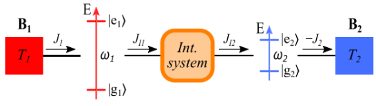
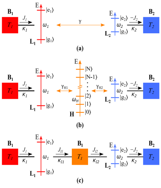
In this notebook, we aim to demonstrate how weak, strong and ultra-strong thermal interactions between quantum thermal devices can be modelled mathematically under three different formalisms, namely a) direct coupling formalism, b) energy divider formalism, c) intermediate bath formalism.To simplify and isolate the essential quantum mechanics of the inter-device interactions, we use a simpler system of two quantum two-level systems (TLSs) interacting with each other, but also with two external thermal baths.The two TLSs play the role of the thermal devices and external baths play the role of the external environment, while the inter-device interactions are modelled as a generic (black-box) intermediate system interacting with them both.
Under each of these formalisms, the intermediate system takes the following forms, respectively.
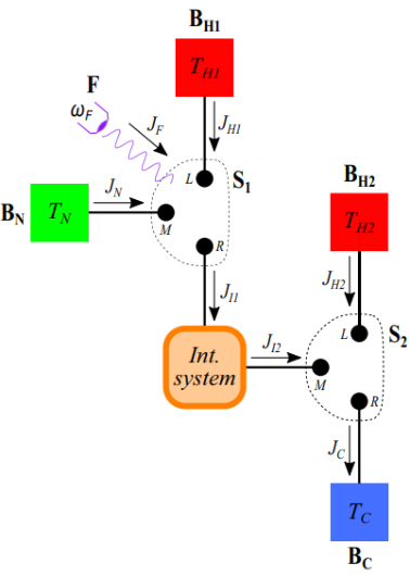
Such interaction models can be used to calculate the thermal flows of multi-device quantum thermal systems, such as the following example of a Darlington pair of quantum thermal transistors.
A more detailed treatment of the underlying physics of these systems can be found in our paper
“Towards quantum thermal multi-transistor systems: Energy divider formalism”, Ravi T. Wijesekara, Sarath D. Gunapala, and Malin Premaratne, Phys. Rev. B 105, 235412 – Published 9 June 2022
“Towards quantum thermal multi-transistor systems: Energy divider formalism”, Ravi T. Wijesekara, Sarath D. Gunapala, and Malin Premaratne, Phys. Rev. B 105, 235412 – Published 9 June 2022
(a) Weak simple direct coupling
In[]:=
BlueC=RGBColor[0.2627,0.4313,1];PurpleC=RGBColor[0.5411,0.0784,0.9607];RedC=RGBColor[0.60,0.30,0];
1. The system has two TLSs coupled each to a thermal bath.
2. The energy levels of the two levels are not necessarily resonant
3. A weak interaction between the two systems mediates the thermal flow from bath to bath.
2. The energy levels of the two levels are not necessarily resonant
3. A weak interaction between the two systems mediates the thermal flow from bath to bath.
Here we take the inter-TLS coupling to be weak. Hence local master equation needs to be used for analysis.
System Hamiltonians
System Hamiltonians
Identity operator
In[]:=
Id[ve_,ho_]:=
δ
ve,ho
Subsystem Hamiltonians
Subsystem Hamiltonians
There are two subsystems L and R, each of which are TLSs.
Combined form for the two non-interacting subsystem Hamiltonians
0
H
sys
ℏ
ω
L
2
e
L
e
L
g
L
g
L
ℏ
ω
R
2
e
R
e
R
g
R
g
R
In[]:=
HLSep[veL_,hoL_,veR_,hoR_]:=
[[veL,hoL]]Id[veR,hoR]HRSep[veL_,hoL_,veR_,hoR_]:=Id[veL,hoL]
[[veR,hoR]]
ℏ ω 1 2 | 0 |
0 | - ℏ ω 1 2 |
ℏ ω 2 2 | 0 |
0 | - ℏ ω 2 2 |
Eigenstates,|1> = |e,e>|2> = |e,g>|3> = |g,e>|4> = |g,g>
Eigenstate mapping function, (maps overall state (1 to 4) to subsystem L, R state,
In[]:=
EmapL[i_]:=+2++1EmapR[i_]:=+2++1
δ
i,3
δ
i,4
δ
i,1
δ
i,2
δ
i,2
δ
i,4
δ
i,1
δ
i,3
Matrix form of the two subsystem Hamiltonians
In[]:=
HL[ve_,ho_]:=HLSep[EmapL[ve],EmapL[ho],EmapR[ve],EmapR[ho]]HR[ve_,ho_]:=HRSep[EmapL[ve],EmapL[ho],EmapR[ve],EmapR[ho]]
Non-interacting subsystem Hamiltonians as a matrix in the combined system space
In[]:=
Hsys0Matrix=Table[HL[ve,ho]+HR[ve,ho],{ve,1,4},{ho,1,4}];MatrixForm[Hsys0Matrix]
Out[]//MatrixForm=
ℏ ω 1 2 ℏ ω 2 2 | 0 | 0 | 0 |
0 | ℏ ω 1 2 ℏ ω 2 2 | 0 | 0 |
0 | 0 | - ℏ ω 1 2 ℏ ω 2 2 | 0 |
0 | 0 | 0 | - ℏ ω 1 2 ℏ ω 2 2 |
Interaction Hamiltonian between the two TLSs
Interaction Hamiltonian between the two TLSs
Combined system Hamiltonian
Combined system Hamiltonian
H
sys
0
H
sys
1
H
sys
In[]:=
HsysMatrix=Hsys0Matrix+Hsys1Matrix;MatrixForm[HsysMatrix]
Out[]//MatrixForm=
ℏ ω 1 2 ℏ ω 2 2 | 0 | 0 | 0 |
0 | ℏ ω 1 2 ℏ ω 2 2 | γℏ 2 | 0 |
0 | γℏ 2 | - ℏ ω 1 2 ℏ ω 2 2 | 0 |
0 | 0 | 0 | - ℏ ω 1 2 ℏ ω 2 2 |
Visualize the energy levels of the combined system
Visualize the energy levels of the combined system
Bare energy levels without the interaction Hamiltonian
Bare energy levels without the interaction Hamiltonian
Function for shifting the eigenvalues from Mathematica to our representation
Dressed energy levels with the interaction Hamiltonian
Dressed energy levels with the interaction Hamiltonian
Function for shifting the eigenvalues from Mathematica to our representation
The interaction Hamiltonian is in the weak regime, hence the energy levels are mostly unchanged by the interaction Hamiltonian.
Density Matrix
Density Matrix
Pauli matrices
Pauli matrices
In z-base representation
In z-base representation
|+z>=(1,0)
|-z>=(0,1)
|-z>=(0,1)
In compound system representation
In compound system representation
Thermal interactions with the baths
Thermal interactions with the baths
Interaction Hamiltonian between the thermal bath L or R with the two TLSs is modelled after the Spin-Boson model in the x-component
Note - Here, P = L, R (or in the simulations P = 1, 2)
The inter-TLS interaction Hamiltonian is supposed to be in the weak regime. The energy eigensystem is minimally affected by the interaction.
This means that it is enough to model the thermal interactions in the bare eigensystem of only the individual TLS Hamiltonians.
This means that it is enough to model the thermal interactions in the bare eigensystem of only the individual TLS Hamiltonians.
Calculating positive transition frequencies
Calculating positive transition frequencies
We work under assumption that energy levels are minimally affected by the interaction term γ.
Assumptions on energy levels
Transition frequencies,
Unique and positive transition frequencies,
Dynamical heat flows
Dynamical heat flows
Thermal distributions in the environments (Bose Einstein distribution),
Characterizing thermal flows
Characterizing thermal flows
Use the first law of thermodynamics, the rate of change of internal energy of the system is equal to the energy inflows
From definition of expected values,
where we used
Substituting the above expression,
Using the relation
we simplify it further
For our particular interaction Hamiltonian, consider the first two terms alone
Therefore we have
Possible definitions for thermal flows
Possible definitions for thermal flows
We can either use the most obvious definition
Or considering that the energy divider terms are relatively weak, we may define
Note how with the second definition a bunch of extra terms comes up. However, all these terms have coefficients
Density matrix, transition rate and energy flow evolution with time
Density matrix, transition rate and energy flow evolution with time
Assumptions on the temperatures of the baths, TLS energy levels, and TLS interaction strengths,
Assumption on the strength of the L-R interaction
System energy matrix under above assumptions,
Numerical solution of the dynamics, with the initial condition that all density matrix elements except the first are zero.
1. For weak interaction strengths (small γ values), the solutions eventually become approximately steady.
2. For fully resonant case, the solutions eventually become completely steady.
2. For fully resonant case, the solutions eventually become completely steady.
Energy flow characteristics for different system parameters
Energy flow characteristics for different system parameters
Energy flow under different levels of resonance
Energy flow under different levels of resonance
Energy flow under different levels of resonance and different coupling strengths
Energy flow under different levels of resonance and different coupling strengths
CITE THIS NOTEBOOK
CITE THIS NOTEBOOK
Towards quantum thermal multi-transistor systems: Energy divider formalism
by Ravi Wijesekara
Wolfram Community, STAFF PICKS, November 16, 2023
https://community.wolfram.com/groups/-/m/t/3066097
by Ravi Wijesekara
Wolfram Community, STAFF PICKS, November 16, 2023
https://community.wolfram.com/groups/-/m/t/3066097