As humans age, intervertebral disks in their spines begin to lose water and reduce the degree to which they can compress, which is known as disk dessication. This in turn reduces the amount their spines are able to move, since the compression is what provides the clearance to move. The most extreme example of this is in Spinal Arthrodesis, where disk compression is circumvented entirely as a way to purposefully restrict movement. By modelling the spine as a simple mechanical model of blocks and springs, the simulation can describe how varying degrees of these conditions can change patients range of motion, using the language of Lagrangian Mechanics to do so. Using Lagrangian Mechanics has the added benefit of helping us easily compute the Range of Motion as a function of the potential energy of the system over time.
Introduction
Introduction
To understand the dynamic behavior of complex mechanical systems, classical physics uses two main approaches, Newtonian mechanics and Lagrangian mechanics. While Newtonian mechanics relies on vectors, which is analyzing individual forces and accelerations for every discrete component, it becomes very complicated and messy when applied to systems with interconnected geometries and kinematic constraints, like those in the spine. Every added joint or constraint introduces new forces (such as normal forces, tensions, and reaction torques) that must be explicitly calculated or isolated through free-body diagrams.
In contrast, Lagrangian mechanics uses the idea scalar energy fields instead of vectors. It uses Hamilton’s Principle of Stationary Action, which states that a system will traverse a path through space that makes the time integral of the Lagrangian function stationary. In other words, the system will try to minimize the distance, force, or anything else, through the idea that things in nature try to take the path of least resistance. The system is characterized by the Lagrangian function L, defined as the difference between the total kinetic energy T and the total potential energy V: L = T - V.
Because the model has 23 segments with biomechanical boundaries, standard force-based physics would require calculating dozens of hidden joint forces. Lagrangian mechanics bypasses these forces entirely by using a streamlined set of coordinates, putting them all into a generalized state vector that describes the system at any given moment in time. To represent the spine biologically, I chose to use a discrete blocks-and-springs model. Vertebrae are treated as rigid blocks, while the flexible discs between them are modeled as axial and torsional springs. This approach allows us to simulate localized spinal conditions, such as disc desiccation (where a disc dries out, loses height, and stiffens) or spinal fusion (where joints are surgically locked together). By simply adjusting the properties of specific springs, I can readily predict how these localized changes alter a patient’s overall range of motion.
Initial Model
Initial Model
In order to model range of motion under these conditions, I must first devise an accurate mechanical simplification of the spine to help us perform computation. I can do this using a series of differential equations, more specifically the Euler-Lagrange equations!
Initializing constants according to literature based values:
In[]:=
n=23;mVal=11;iVal=0.00003;kVal=850;bVal=0.16Sqrt[mVal*kVal];l0Val=1.0;tMax=3;
Consider a system composed of 23 interconnected segments, each with 3 degrees of freedom (DOF); x, y, and θ, but with 1 locked base segment.
Creating functions for each DOF, and their velocities as the first derivative:
In[]:=
q=Flatten[Table[{x[i][t],y[i][t],θ[i][t]},{i,n}]];dq=D[q,t];q//Shortdq//Short
Out[]//Short=
{x[1][t],y[1][t],θ[1][t],x[2][t],61,θ[22][t],x[23][t],y[23][t],θ[23][t]}
Out[]//Short=
{[t],[t],[t],63,[t],[t],[t]}
′
x[1]
′
y[1]
′
θ[1]
′
x[23]
′
y[23]
′
θ[23]
Assuming the connections are governed by elastic restoring forces (springs), the force F exerted by an individual spring follows Hooke’s Law:
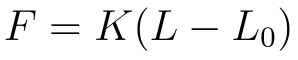
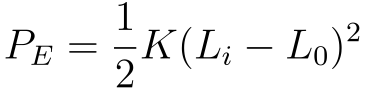
where K is the spring constant, L is the current length, and is the natural un-stretched length. Integrating this force with respect to the displacement yields the potential energy stored in a single spring element:
L
0
P
E
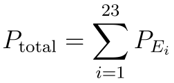
For a system of 23 segments, the total potential energy is obtained by summing the individual potential energies:
P
total
And equivalently in Wolfram Language, with the hypotenuse of the x and y position of the given segment representing its present spring length,
Sum of potential energies of each segment:
In[]:=
p=1/2*kVal*(Sqrt[x[1][t]^2+y[1][t]^2]-l0Val)^2+Sum[1/2*kVal*(Sqrt[(x[i+1][t]-x[i][t])^2+(y[i+1][t]-y[i][t])^2]-l0Val)^2,{i,n-1}];p//Short
Out[]//Short=
425+425+19+425+425
2
-1.++
2
111]
2
1
2
(1)
2
1
2
(-1.+
1+1
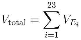
)To compute the Lagrangian, I also need to find the total kinetic energy of the overall system over time. The kinetic energy for the i-th individual segment is the sum of its translational and rotational kinetic energies:
V
E
i

Where is the mass of the i-th segment, is its moment of inertia, and the overdots denote time derivatives, (=).Summing across all 23 segments provides the total kinetic energy of the system.
m
i
I
i
x
dx
dt
V
total
The code to perform the same computation in Wolfram language is as follows.
Sum of kinetic energies of each segment:
In[]:=
v=Sum[1/2*mVal*(D[x[i][t],t]^2+D[y[i][t],t]^2)+1/2*iVal*D[θ[i][t],t]^2,{i,n}];v//Short
Out[]//Short=
11
2
2
′
x[1]
2
′
y[1]
2
′
1
In order for the system to be anatomically accurate, it must also include damping. In fact, one of the primary functions of the spine is to absorb and redistribute force throughout the body, so as to not put too much stress on any one joint. This makes the Euler-Lagrange equation angry, since we are effectively ruining the relationship between the kinetic and potential energies in the Lagrangian by absorbing some energy in the damping. I can get around this using an external dissipation function though, which in this case will be the Rayleigh Dissipation function:
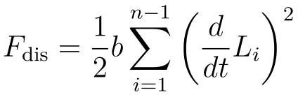
In Wolfram Language, this looks like,
Implement Rayleigh dissipation function
In[]:=
fdis=Sum[1/2*bVal*(D[x[i][t],t]^2+D[y[i][t],t]^2+D[θ[i][t],t]^2),{i,n}];
To help us compute the differential equations a bit cleaner, I have to use a symbolic interpretation of every equation and derivative I am solving for.
Create symbols and associations to reformat and input later:
In[]:=
qSym=Flatten[Table[{Symbol["x"<>ToString[i]],Symbol["y"<>ToString[i]],Symbol["θ"<>ToString[i]]},{i,n}]];dqSym=Flatten[Table[{Symbol["dx"<>ToString[i]],Symbol["dy"<>ToString[i]],Symbol["dθ"<>ToString[i]]},{i,n}]];toSym=Join[Thread[q->qSym],Thread[dq->dqSym]];toFunc=Join[Thread[qSym->q],Thread[dqSym->dq]];vSym=v/.toSym;pSym=p/.toSym;fdisSym=fdis/.toSym;
Evaluating Model
Evaluating Model
I have all of the prerequisites! I can now make a list of the equations to solve.
Make a list of equations using the symbols made:
In[]:=
eqs=Table[D[D[vSym,dqSym[[j]]]/.toFunc,t]-(D[vSym,qSym[[j]]]/.toFunc)+(D[pSym,qSym[[j]]]/.toFunc)+(D[fdisSym,dqSym[[j]]]/.toFunc)==0,{j,Length[q]}];
I can do the same thing for the initial conditions, which describe the position and velocity each section will take on at t = 0.
Make a list of initial conditions:
In[]:=
ics=Flatten[Table[{y[i][0]==i*l0Val,θ[i][0]==0,x[i][0]==i*Tan[iDegree],x[i]'[0]==-1.4i*Tan[iDegree],y[i]'[0]==0,θ[i]'[0]==1000},{i,n}]];ics//Short
Out[]//Short=
{y[1][0]1.,θ[1][0]0,134,[0]0,[0]1000}
′
y[23]
′
θ[23]
It also needs a list of dependent variables to satisfy NDSolve.
Make a list of all dependent variables to solve for:
In[]:=
dependentVariables=Flatten[Table[{x[i],y[i],θ[i]},{i,n}]];dependentVariables//Short
Out[]//Short=
{x[1],y[1],θ[1],x[2],y[2],θ[2],57,x[22],y[22],θ[22],x[23],y[23],θ[23]}
Use NDSolveValue to get the parametric interpolated functions:
In[]:=
solutions=NDSolveValue[Join[eqs,ics],dependentVariables,{t,0,tMax}];solutions//Short
Out[]//Short=
InterpolatingFunction,67,InterpolatingFunction


I can now assign the first block to constant values so it doesn’t move.
Define constant values for the first block, and solved values for the rest:
ClearAll[xSol,ySol,θSol]xSol[1,t_]:=0.0;ySol[1,t_]:=1.0;θSol[1,t_]:=0.0;xSol[i_,t_]:=solutions[[3(i-1)+1]][t]ySol[i_,t_]:=solutions[[3(i-1)+2]][t]θSol[i_,t_]:=solutions[[3(i-1)+3]][t]
I can animate the solution now!
Create an animation of rectangles based on the equations:
As shown in the animation, the initial velocity applied to the rectangles is proportional to its position, and the forces that come with it are also distributed over time through the system. Note the slinky-like movement of the spine as it absorbs the forces from the uppermost segment. However, this model is still inaccurate. The masses on each spring are being represented as single points with mass, meaning rotational velocity has no bearing on any of the rectangles. The rectangles and springs also have no concrete attachments, as the rectangles are merely visual artifacts from the animation. Mathematically grounding the rectangles means adding torsional spring resistance and axial and angle barriers, and a lot more to approach realism. I have my work cut out for me!
Advanced Model
Advanced Model
Consider another system composed of 23 interconnected segments, each with 3 DOF; x, y, and θ, but with 1 locked base segment, and with the 23rd segment locked on an arc to prevent collapse. The more realistic model involves a lot more constants now. There are defined variables for the width and height of the vertebrae, for gravity, two values for limits on axial compression and angular compression, and a new arbitrarily high value for maximum joint angle.
Real spines also have different sections contribute different amounts to lateral bending motion than others. Because of this, the spring constants can be graded accordingly, using simple decay to assign decreasing values to higher segments. I also included a torsional spring constant to resist rotation from the blocks above and below, which helps visualize a more realistic spine.
Define top and bottom spring constants, and use decay for constants in between:
I can take the liberty to lock the first segment of the spine since I am modelling the spine in isolation; in reality, it would be surrounded by tissue and tendons, and would have the pelvis and legs beneath it.
Lock the L1 base segment:
Define the arc that the top segment follows:
Interpreting these equations into Wolfram language is as follows,
Attach springs to tops and bottoms of rectangles:
The deformation and separation of the attached springs:
I can do the same exercise from before of defining all of the equations and derivatives to solve for, this time with phi for the 23rd segment.
Define equations to solve for:
Next, I find the total potential energy again with the same regular spring potential energy, but this time with finding the sum of the torsional spring forces using Hooke’s Law for Rotation,
gravity,
axial compression,
and angular compression.
Translating this into Wolfram Language,
Sum of all potential energies:
Calculating the kinetic energy and dissipation is quite similar to last time.
Sum of kinetic energy, and sum of energy loss from damping:
Now that I have the Potential and Kinetic Energy, I can use the Lagrangian to make the equations of motion. The general formula is as follows,
Euler-Lagrange equations for the system, per block:
Evaluating Model
Evaluating Model
I can define the initial positions based on the equations of motion from before.
Define initial conditions and append them to total solver list:
Now I solve for the interpolating functions!
Use NDSolve to track rectangle position over time:
Because of certain coordinates I left out in the solver, I have to define functions to reconstruct the proper mappings needed for the animation. Again, I lock the first block,
Lock the first block at (0,0,0):
And also sort the equations into their respective DOF,
Sort the remaining equations to the DOF they solve for:
This time though, I have to also define specific values for the uppermost block, using phi and a radius to describe how it moves in the x and y.
Explicitly define how the top block can move:
Now I can animate the new system!
Analysis
Analysis
To evaluate how the spinal column moves dynamically, I tracked the absolute spatial joint angles over time, and plotted them across the simulation window.
Plot the joint angles of each segment in terms of the plane over time:
When the simulation initializes, gravity pulls downward on the segments and the top boundary block is forced along its orbital track. This triggers an aggressive transient phase where the spine undergoes large and erratic oscillations. Because the system incorporates Rayleigh damping, these wild movements steadily bleed out energy, causing the oscillations to decay until the spine settles into a stable, damped harmonic steady-state.
I can extract an average value of all of the minima of these curves, to help generalize the joint angles over time of systems with different constants.
Compute average minima of all curves in a given system:
Next, I simulated the mechanical consequences of spinal arthrodesis (surgical joint fusion). Multiple trials were executed, which sequentially locked an increasing number of intervertebral joints, and mapped the number of fused joints against the average of the maximum Range of Motion (ROM) observed across all 23 segments. The purpose of these trials was to see how varying degrees of fusion, would help or hurt the range of motion.
Create points for the data, and generalize to a curve:
Plot the new relation:
The 2D scatterplot shows a inversely proportional downward trend, wherein the number of fused joints increases as the average maximum ROM of each segment drops. When you fuse a joint, its own local flexibility is driven to zero, which naturally drags down the mathematical average of the entire kinematic chain.
This graph can also be interpreted as showing the trade-off of spinal fusion surgery. While locking unstable vertebrae can help eliminate painful micro-movements, it hurts macro-level flexibility. In clinical practice, this loss of mobility forces the remaining, healthy joints to overcompensate by bending further. Over time, this localized tension subjects the healthy discs to excessive stress, accelerating their degeneration, which causes a major clinical condition known as Adjacent Segment Disease (ASD).
The spine often distributes movement differently than normal during lateral bending, where the lumbar spine and lower thoracic have different degrees to which they bend. To analyze how this layout determines overall flexibility, I conducted a very simplified parametric sensitivity analysis across simulation trials, mapping the results onto a 3D scatterplot.
Create a list of points to plot, based on gathered experimental data from the simulation:
Graph the set of gathered points:
Our simulation is very accurate! It is able to correctly show the expected relationship between the axial compression and torsional compression, and how making the intervertebral disks stiffer reduces our mean range of motion. It is also evident that making the disks stiffer has “diminishing returns”, meaning it takes a bigger jump in stiffness to get from 0.5 radians of rotation to 0.4 radians than it does to go from 0.6 to 0.5. Expanding our dataset to a more robust amount of trials would more than likely return a curve that would verify these same results.
Conclusion
Conclusion
In this project, I have developed two physics simulations of the spine, with which I was able to explore how disk dessication and spinal fusion affect the spine’s range of motion. I learned and used Lagrangian mechanics to generate the motion of the spines I made, which allowed easier calculations and a more systematic approach to calculating the equations of motion that described the spine. Our results show that increasing the amount of fused segments and the stiffness between disks has a negative correlation to range of motion in terms of their joint angles in space. and In creating these models and comparing how they moved when initialized with different constants, I was able to show the negative impact arthrodesis and desiccation can have on patient’s range of motion, which could also be applied to other similar spinal conditions that affect range of motion.
Future Directions
Future Directions
Future work on this project could involve improving upon the spinal systems by using a more comprehensive model of each intervertebral disk, namely the Standard Linear Solid or Standard Nonlinear Solid viscoelastic model of the disk. Another natural extension is to extend these models into 3 dimensions, which could build off of the existing model easily by adding more degrees of freedom. Finally, introducing irregular, vertebrae-shaped elements instead of regular rectangles would add another degree of complexity and realism to the physics and interactions within the model.
Acknowledgements
Acknowledgements
I would like to thank to thank my mentor Junseo Lee for helping me so much throughout the project and for sifting through my ramblings together. Thank you to Joseph Brennan for helping me with my physics questions and grounding my thinking. Thank you to Bryan, Divya, Amrita, Arnay, Eric, and all of the TA’s for keeping things fun and helping me consider new ideas. I would like to thank Rory Foulger, Megan Davis, and Eryn Gillam for creating such a fantastic research environment. I would also like to thank Stephen Wolfram for the great conversations at this program and his continued support throughout the project process.
Additional thanks to Stephen Wolfram for suggesting this project.
Citations
Citations
◼
Edmondston, S. J., Aggerholm, M., Elfving, S., Flores, N., Ng, C., Smith, R., & Netto, K. (2007). Influence of posture on the range of axial rotation and coupled lateral flexion of the thoracic spine. Journal of Manipulative and Physiological Therapeutics, 30(3), 193–199. https://doi.org/10.1016/j.jmpt.2007.01.010
◼
Morin, D. (n.d.). The lagrangian method. Institute of Physics and Chemistry of Materials of Strasbourg. Retrieved https://www.ipcms.fr/uploads/2021/06/chap6.pdf
◼
NDSolveValue: Solve a differential equation numerically—Wolfram Documentation. (n.d.). Retrieved July 9, 2026, from https://reference.wolfram.com/language/ref/NDSolveValue.html?q=NDSolveValue
◼
Simple harmonic oscillator equation. (n.d.). Retrieved July 9, 2026, from https://farside.ph.utexas.edu/teaching/315/Waveshtml/node5.html
◼
Weisstein, E. W. (n.d.). Euler-lagrange differential equation [Text]. Retrieved July 9, 2026, from https://mathworld.wolfram.com/Euler-LagrangeDifferentialEquation.html
◼
[Wss23] interactive demonstration of lagrangian mechanics—Online technical discussion groups—Wolfram community. (n.d.). Retrieved July 9, 2026, from https://community.wolfram.com/groups/-/m/t/2959079
CITE THIS NOTEBOOK
CITE THIS NOTEBOOK
Range of motion during disk desiccation and spinal arthrodesis using Lagrangian mechanics
by Ahaan Gupta
Wolfram Community, STAFF PICKS, July 9, 2026
https://community.wolfram.com/groups/-/m/t/3752279
by Ahaan Gupta
Wolfram Community, STAFF PICKS, July 9, 2026
https://community.wolfram.com/groups/-/m/t/3752279