This Mathematica script implements a full liquid-liquid equilibrium (LLE) phase-split calculation using the NRTL activity coefficient model, parameterized for the quaternary system {Water (1) + Ethanol (2) + 2-Propanol (3) + Isooctane (4)} at 308.2 K, using the binary interaction parameters reported by de Klerk and Schwarz (2022). The foundation of the code is the tau[i,j,T] and G[i,j,T] functions, which compute the temperature-dependent NRTL binary interaction parameters and the corresponding Boltzmann-type weighting factors. These feed into lnGamma[i,x,T], which implements the full multicomponent NRTL activity coefficient expression (summing local-composition contributions over all species), and its exponentiated counterpart gamma[i,x,T], giving the actual activity coefficient of component i for any mole-fraction vector and temperature.
The first major analytical tool built on top of this model is the Tangent Plane Distance (TPD) function, TPD[w1,w2,w3], which evaluates the thermodynamic stability of a trial composition w relative to a fixed overall (feed) composition z. The TPD is defined as the difference between the Gibbs energy of a candidate phase and the tangent plane to the Gibbs surface at the feed composition; a negative TPD value at the global minimum indicates that the homogeneous feed is thermodynamically unstable and will split into two liquid phases. This is the standard global stability analysis approach for verifying that a system is genuinely biphasic before attempting an equilibrium (tie-line) calculation, rather than a single homogeneous phase.
For each experimental tie line being tested (the code processes several, labeled POINT 1, POINT 2, POINT 3), the workflow begins by averaging the two reported experimental conjugate-phase compositions to define the overall feed composition z. NMinimize is then used with the Differential Evolution algorithm to find the global minimum of the TPD function over the composition simplex, returning both the minimum TPD value and the corresponding most unstable trial composition. A TPD minimum significantly below zero confirms phase splitting is thermodynamically favored and gives an initial guess for one of the two equilibrium phases.
The second stage solves the actual phase-split (flash) equations via the eqns[...] function, which encodes the isofugacity (equal activity × mole fraction) conditions between the two liquid phases for components 1–3, along with Rachford-Rice-style mass balance equations relating each phase’s composition to the overall feed z through the phase fraction beta (the fraction of feed in the “raffinate”/Phase B). The system uses the K-values (ratio of activity coefficients between phases) inside a Rachford-Rice residual rr, ensuring overall mass balance closure across all four components simultaneously with the phase-fraction variable. An initial guess for one phase is taken from the TPD result, and the conjugate phase composition is backed out via the overall mass balance using an assumed betaGuess.
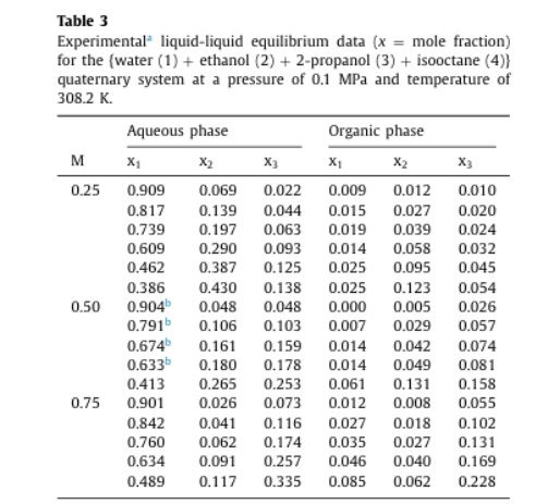
Finally, FindRoot is used to simultaneously solve this nonlinear system of seven equations for seven unknowns (three independent mole fractions in each of two phases, plus beta), refining the initial guesses into a converged, thermodynamically consistent tie-line solution. This is repeated independently for each experimental tie-line point, allowing direct comparison between the NRTL-model-predicted phase split (composition of both liquid phases and the phase fraction beta) and the experimentally measured tie lines reported in the original paper — effectively validating how well the regressed NRTL parameters reproduce the measured quaternary LLE behavior at 308.2 K (see Table 3 of Ref. 1).
NRTL Binary Interaction Parameters System:{Water (1)+Ethanol (2)+2-Propanol (3)+Isooctane (4)}
Source:de Klerk& Schwarz,Fluid Phase Equilibria 556 (2022) 113407,Table 6 Valid temperature range:298.2 K to 328.2 K
Model form:tau[i,j]=a[i,j]+b[i,j]/T G[i,j]=Exp[-alpha[i,j]*tau[i,j]]
Source:de Klerk& Schwarz,Fluid Phase Equilibria 556 (2022) 113407,Table 6 Valid temperature range:298.2 K to 328.2 K
Model form:tau[i,j]=a[i,j]+b[i,j]/T G[i,j]=Exp[-alpha[i,j]*tau[i,j]]
Component index map
components=<|1->"Water",2->"Ethanol",3->"2-Propanol",4->"Isooctane"|>;
Non-randomness parameters alpha[i,j]=alpha[j,i]
alpha=<|{1,2}->0.3,{2,1}->0.3,{1,3}->0.3,{3,1}->0.3,{1,4}->0.2,{4,1}->0.2,{2,3}->0.3,{3,2}->0.3,{2,4}->0.47,{4,2}->0.47,{3,4}->0.3,{4,3}->0.3|>;
Temperature-independent coefficients a[i,j] (dimensionless)
aPar=<|{1,2}->-14.146,{2,1}->-1.150,{1,3}->9.764,{3,1}->-2.484,{1,4}->-21.132,{4,1}->-6.494,{2,3}->0.135,{3,2}->0.701,{2,4}->-3.029,{4,2}->-5.381,{3,4}->-3.469,{4,3}->1.929|>;
Temperature-dependent coefficients b[i,j] (units:K)
bPar=<|{1,2}->5751.7,{2,1}->-190.0,{1,3}->-2320.0,{3,1}->571.1,{1,4}->9893.0,{4,1}->3162.6,{2,3}->-215.7,{3,2}->-58.4,{2,4}->1417.5,{4,2}->2113.7,{3,4}->1344.6,{4,3}->-447.0|>;
tau[i,j] as a function of temperature T (in Kelvin)
tau[i_,j_,T_]:=aPar[{i,j}]+bPar[{i,j}]/T
G[i,j] as a function of temperature T
G[i_,j_,T_]:=Exp[-alpha[{i,j}]*tau[i,j,T]]
tau[i,i]=0 and G[i,i]=1 by convention
tau[i_,i_,T_]:=0G[i_,i_,T_]:=1
NRTL activity coefficient (Eq.2 in the paper)
lnGamma[i_,x_List,T_]:=Module[{n=Length[x]},Sum[tau[j,i,T]*G[j,i,T]*x[[j]],{j,n}]/Sum[G[k,i,T]*x[[k]],{k,n}]+Sum[(G[i,j,T]*x[[j]])/Sum[G[k,j,T]*x[[k]],{k,n}]*(tau[i,j,T]-Sum[tau[l,j,T]*G[l,j,T]*x[[l]],{l,n}]/Sum[G[k,j,T]*x[[k]],{k,n}]),{j,n}]]gamma[i_,x_List,T_]:=Exp[lnGamma[i,x,T]]
In[]:=
T=308.2;
In[]:=
Clear[TPD];TPD[w1_?NumericQ,w2_?NumericQ,w3_?NumericQ]:=Module[{w4,w,gammaW},w4=1-w1-w2-w3;If[w1<=0||w2<=0||w3<=0||w4<=0,Return[10^10]];w={w1,w2,w3,w4};gammaW=Table[gamma[i,w,T],{i,1,4}];Sum[w[[i]]*(Log[w[[i]]*gammaW[[i]]]-Log[z[[i]]*gamma[i,z,T]]),{i,1,4}]];
Point 1 - tie line
In[]:=
xPhaseI={0.462,0.387,0.125,1-0.462-0.387-0.125};xPhaseII={0.025,0.095,0.045,1-0.025-0.095-0.045};z=(xPhaseI+xPhaseII)/2;zTotal[z]
Out[]=
{0.2435,0.241,0.085,0.4305}
Out[]=
1.
In[]:=
sol=NMinimize[{TPD[w1,w2,w3],w1>=10^-6,w2>=10^-6,w3>=10^-6,1-w1-w2-w3>=10^-6},{w1,w2,w3},Method->{"DifferentialEvolution"}];TPDmin=sol[[1]];Print[" TPDmin = ",NumberForm[TPDmin,{12,8}]]
TPDmin = -0.11828958
In[]:=
sol
Out[]=
{-0.11829,{w10.609014,w20.323,w30.0600697}}
ClearAll[eqns];eqns[xa1_,xa2_,xa3_,xb1_,xb2_,xb3_,beta_]:=Module[{xa4,xb4,xa,xb,ga,gb,K,rr},xa4=1-xa1-xa2-xa3;xb4=1-xb1-xb2-xb3;xa={xa1,xa2,xa3,xa4};xb={xb1,xb2,xb3,xb4};ga=Table[gamma[i,xa,T],{i,1,4}];gb=Table[gamma[i,xb,T],{i,1,4}];K=ga/gb;rr=Sum[z[[i]]*(K[[i]]-1)/(1+beta*(K[[i]]-1)),{i,1,4}];{xa[[1]]*ga[[1]]-xb[[1]]*gb[[1]],xa[[2]]*ga[[2]]-xb[[2]]*gb[[2]],xa[[3]]*ga[[3]]-xb[[3]]*gb[[3]],xa[[1]]-z[[1]]/(1+beta*(K[[1]]-1)),xa[[2]]-z[[2]]/(1+beta*(K[[2]]-1)),xa[[3]]-z[[3]]/(1+beta*(K[[3]]-1)),rr}];
In[]:=
betaGuess=0.65
Out[]=
0.65
In[]:=
xbGuess={0.6090,0.3230,0.06006};(*fromTPD*)(*backoutxafrommassbalanceusingnormalizedz*)xaGuess=(z[[1;;3]]-(1-betaGuess)*xbGuess)/betaGuess;
In[]:=
xaGuess
Out[]=
{0.0466923,0.196846,0.0984292}
In[]:=
solRoot=FindRoot[eqns[xa1,xa2,xa3,xb1,xb2,xb3,beta],{{xa1,xaGuess[[1]]},{xa2,xaGuess[[2]]},{xa3,xaGuess[[3]]},{xb1,xbGuess[[1]]},{xb2,xbGuess[[2]]},{xb3,xbGuess[[3]]},{beta,betaGuess}},MaxIterations->1000]
Out[]=
{xa10.0217695,xa20.0728027,xa30.0587541,xb10.455904,xb20.402123,xb30.110142,beta0.510741}
POINT 2
In[]:=
xPhaseI={0.760,0.062,0.174,1-0.760-0.062-0.174};xPhaseII={0.035,0.027,0.131,1-0.035-0.027-0.131};z=(xPhaseI+xPhaseII)/2;zTotal[z]
Out[]=
{0.3975,0.0445,0.1525,0.4055}
Out[]=
1.
In[]:=
sol=NMinimize[{TPD[w1,w2,w3],w1>=10^-6,w2>=10^-6,w3>=10^-6,1-w1-w2-w3>=10^-6},{w1,w2,w3},Method->{"DifferentialEvolution"}];TPDmin=sol[[1]];Print[" TPDmin = ",NumberForm[TPDmin,{12,8}]]
TPDmin = -0.37615261
In[]:=
sol
Out[]=
{-0.376153,{w10.961252,w20.0104016,w30.028232}}
ClearAll[eqns];eqns[xa1_,xa2_,xa3_,xb1_,xb2_,xb3_,beta_]:=Module[{xa4,xb4,xa,xb,ga,gb,K,rr},xa4=1-xa1-xa2-xa3;xb4=1-xb1-xb2-xb3;xa={xa1,xa2,xa3,xa4};xb={xb1,xb2,xb3,xb4};ga=Table[gamma[i,xa,T],{i,1,4}];gb=Table[gamma[i,xb,T],{i,1,4}];K=ga/gb;rr=Sum[z[[i]]*(K[[i]]-1)/(1+beta*(K[[i]]-1)),{i,1,4}];{xa[[1]]*ga[[1]]-xb[[1]]*gb[[1]],xa[[2]]*ga[[2]]-xb[[2]]*gb[[2]],xa[[3]]*ga[[3]]-xb[[3]]*gb[[3]],xa[[1]]-z[[1]]/(1+beta*(K[[1]]-1)),xa[[2]]-z[[2]]/(1+beta*(K[[2]]-1)),xa[[3]]-z[[3]]/(1+beta*(K[[3]]-1)),rr}];
In[]:=
betaGuess=0.495
Out[]=
0.495
In[]:=
xaGuess={w1,w2,w3}/.sol[[2]](*fromTPD*)(*backoutxbfrommassbalanceusingnormalizedz*)xbGuess=(z[[1;;3]]-(1-betaGuess)*xbGuess)/betaGuess;
Out[]=
{0.961252,0.0104016,0.028232}
In[]:=
xbGuess
Out[]=
{-0.17764,0.0792872,0.279278}
In[]:=
solRoot=FindRoot[eqns[xa1,xa2,xa3,xb1,xb2,xb3,beta],{{xa1,xaGuess[[1]]},{xa2,xaGuess[[2]]},{xa3,xaGuess[[3]]},{xb1,xbGuess[[1]]},{xb2,xbGuess[[2]]},{xb3,xbGuess[[3]]},{beta,betaGuess}},MaxIterations->1000]
Point 4
References
References
[1] de Klerk, D. L., & Schwarz, C. E. (2022). Quaternary liquid-liquid equilibria measurements and NRTL modelling for the (Water + Ethanol + 2-Propanol + 2,2,4-Trimethylpentane) system at 298.2K to 328.2K. Fluid Phase Equilibria, 556, 113407. https://doi.org/10.1016/j.fluid.2022.113407
CITE THIS NOTEBOOK
CITE THIS NOTEBOOK
Liquid-liquid phase split calculations for the water + ethanol + 2-propanol + iso-octane system
by Housam Binous
Wolfram Community, STAFF PICKS, June 27, 2026
https://community.wolfram.com/groups/-/m/t/3740133
by Housam Binous
Wolfram Community, STAFF PICKS, June 27, 2026
https://community.wolfram.com/groups/-/m/t/3740133