Abstract: Hackenbush is a class of two-player zero-sum perfect information games. It is played on a graph whose edges are available to either or both players for removal. Players alternate in removing edges of the graph. After each removal, any edges unconnected to a distinguished vertex are removed from the graph. In the standard version of the game, the first player without any available moves loses. We explore Hackenbush games by constructing multiway graphs corresponding to all possible sequences of moves. Using this multiway graph, we determine the winning player at each position, and determine the probability for each player to win when they pick their moves randomly. Future work on Hackenbush can build on our framework to determine the (Conway-)value of Hackenbush graphs.
(Hint: If some titles sound an odd bell, try if they are links!)
1.1 First steps in non-violent, finite Hackenbush (with machetes)
1.1 First steps in non-violent, finite Hackenbush (with machetes)
We won’t talk much about the history of Hackenbush. In a way, it’s mainly Conway’s fault [1]. Others are culpable for the methodology we aim to follow.
Here’s how you play Hackenbush. You need two players, Blue and Red.
Here’s how you play Hackenbush. You need two players, Blue and Red.
In[]:=
stickHuman[color_]:=Graphics[Style[{Circle[{0,5},1],Line[{{0,4},{0,1}}],Line[{{0,3},{2,4}}],Line[{{0,3},{-2,4}}],Line[{{0,1},{1.5`,-1}}],Line[{{0,1},{-1.5`,-1}}]},color,Thickness[0.05`]],ImageSizeTiny];GraphicsRow[{stickHuman[Blue],stickHuman[Red]},Scaled[0.3]]
Out[]=
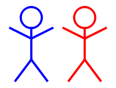
Both Blue and Red are equipped with a machete.
In[]:=
machete[color_]:=ImageResizeColorReplaceBinarize
,{Blackcolor},70;GraphicsRow[{stickHuman[Blue],machete[Blue],ImageReflect[machete[Red],Left],stickHuman[Red]},Scaled[0.3]]

Out[]=
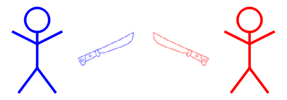
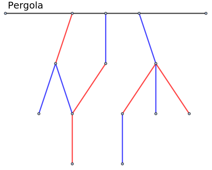
Despite early appearances, there is little space for direct violence in Hackenbush. Blue and Red are hacking away at the edges of a ‘bush’. The edges can be Red or Blue (and, later, Green) and will be represented with a colored graph.
In[]:=
assignColor[actionSet_,color_]:=Append[#,color]&/@actionSet;edgesColored[acts_]:=UndirectedEdge@@@Flatten[Union[assignColor[acts[#],#]&/@{Blue,Red,Green}],1];actions[Blue]={{2,5},{3,6},{4,7},{4,8},{6,10},{9,13}};actions[Red]={{1,4},{5,8},{6,9},{6,11},{8,12}};actions[Green]={};GraphedgesColored[actions],VertexCoordinates->,EdgeStyle->{x_:>Last[x],Thick}
Out[]=
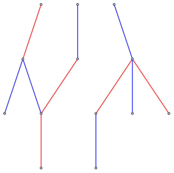
The bush-graph hangs from a pergola...
In[]:=
ImageResize[WikipediaData["Pergola","ImageList"][[12]],Medium]
Out[]=
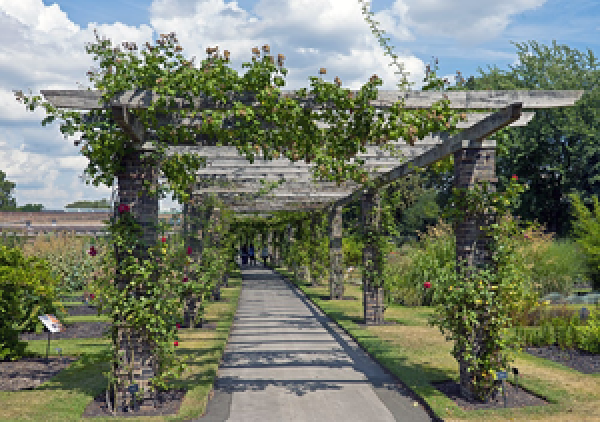
...like this:
Out[]=
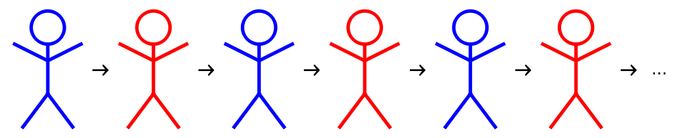
One of the players starts. Players move sequentially, that is, either Blue first:
In[]:=
GraphicsRow[Riffle[Append[Flatten[Table[stickHuman/@{Blue,Red},3]],Style["...",12]],Style["→",15]],Scaled[0.3]]
Out[]=
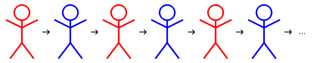
or Red first:
In[]:=
GraphicsRow[Riffle[Append[Flatten[Table[stickHuman/@{Red,Blue},3]],Style["...",12]],Style["→",15]],Scaled[0.3]]
Out[]=
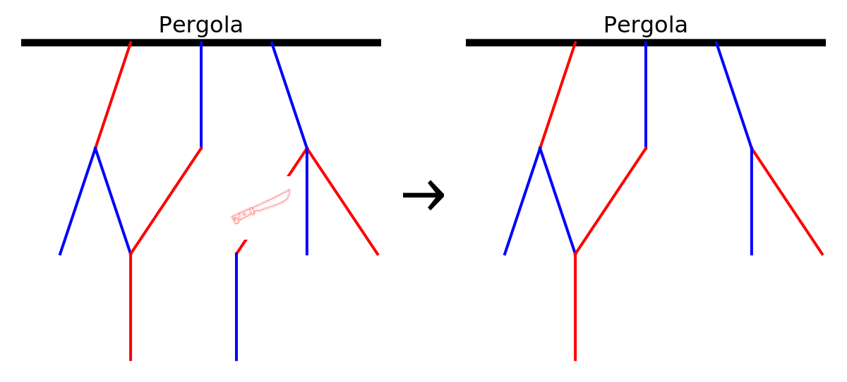
On their turn, each player needs to remove one of the edges matching their color, or a green one. That is, the Blue player can cut Blue and Green edges, and the Red Player can cut Red and Green ones.
In[]:=
GraphicsRow[Flatten[Riffle[{stickHuman[#[[1]]],machete[#[[1]]],Graphics[Style[Line[{{0,0},{1,-0.5}}],#[[2]]],ImageSize->Tiny]}&/@{{Blue,Blue},{Blue,Green},{Red,Red},{Red,Green}},Style[" or ",20]]],Spacings->20,ImageSize{800,100}]
Out[]=

After the edge is removed, any edges (of either color) that became disconnected from the pergola ‘fall off’, and are also removed from the game.
In[]:=
Out[]=
Out[]=
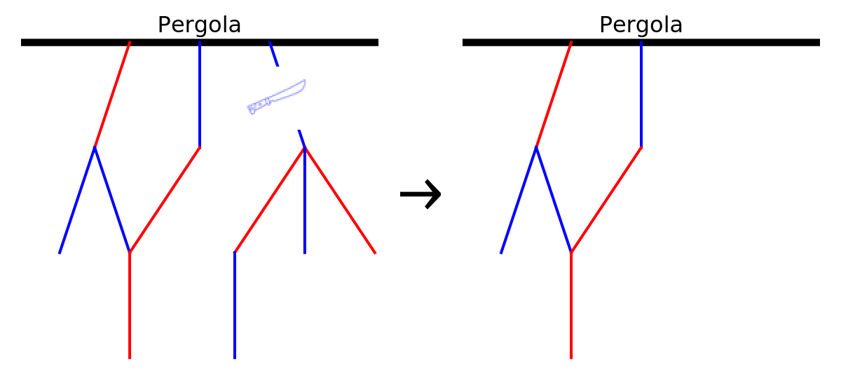
The first player who cannot remove an edge on their turn loses.
For example, in this game state, if it is Red‘s turn, they lose - conversely, Blue wins:
For example, in this game state, if it is Red‘s turn, they lose - conversely, Blue wins:
Note that there' s no score, or any qualification to victory and loss,
1.2 ...to draw fewer pergolas and machetes
1.2 ...to draw fewer pergolas and machetes
We aim to find the simplest representation of a Hackenbush game. First, notice that nothing in game changes if all the edges connected to the pergola meet at one point/vertex:
We don’t really need the bar representing the pergola - we just need to highlight the point/vertex representing it. We number this vertex as 1. To be able to refer to the vertices and edges, we number all the others, too.
This representation seems simple, and includes all the information we need.
1.3 Non-random and random bush-growth
1.3 Non-random and random bush-growth
Repeating from above, this is how we assign color to the edges of our graph:
We define a style...
and a way to generate each game’s graph directly from the list of possible actions.
To specify a Hackenbush game, we need two ingredients: the game graph, and the specification of the player whose turn it is - sometimes we will refer to it as the ‘current’ player. We opt to use an association:
Note that this structure can be used to encode not only the initial state, but any position reached after a (finite) sequence of moves. We will sometimes call these positions ‘game states’. There is no crucial difference between a Hackenbush game state reached after some moves, and a Hackenbush game that starts just now from the same position, with the same starting player as whose turn it is. (We could say that Hackenbush is ‘Markovian’. Many chess positions - understood as only the current position of the pieces on the board -, by the way, are not so, due to the en passant and castling rules).
With these functions at hand, generating a game is simple.
To generate random games, we take three parameters:
1. the number of vertices in the game,
2. the list of Red, Blue, and Green edges, and
3. an optional random-seed value.
Our function checks that the vertex count and the total number of edges is compatible: too few vertices, and we can’t connect them all to the pergola. And too many vertices just won’t fit.
We generate a random graph until it is connected - otherwise, we’d lose some edges right from the start of the game. We scramble their order, and then color them. The starting player is also chosen randomly.
The return value is an association, according to the convention adopted above.
The default seed value returns the same game as the one we constructed above:
2. Groughs Through (All Possible) Rough Troughs
2. Groughs Through (All Possible) Rough Troughs
2.1 Shapes of moving hacks
2.1 Shapes of moving hacks
Making a move means removing the chosen edge, and then all other edges that fall off. ConnectedGraphComponents[] helps us here.
We can list all possible moves from a game state: these are the edges corresponding to the current player’s color, plus the green edges.
In this game, Red has 10 moves:
Using this, we can make moves randomly:
2.2 All your plays belong on a graph
2.2 All your plays belong on a graph
We want to map out all possible sequences of moves. To start, we create a list of all possible `next’ game states.
In this game, Red has three possible moves:
And so we get three possible game states after one move.
We can iterate NestWhileGraph to generate all possible sequences of moves. This is sometimes called the \b’game graph’. We will color the vertices of this graph according to which players’ turn it is. We also highlight the node corresponding to the start of the game.
In this game graph, nodes correspond to game states. Arrows represent single moves, leading from a game state to another one (where the arrows point) - hence the directedness of the graph. Because each Hackenbush move reduces the size of the bush by at leas End-states correspond to nodes from which no
2.3 Canonical (W.) Bushes
2.3 Canonical (W.) Bushes
The decision to label the vertices by numbers in Section 1.2 was not entirely innocuous. For example, these g0 and g1 below clearly correspond to the same Hackenbush game state:
However, the graphs are not the same:
So when we map out all possible plays using makeGameGraph, it may happen that what is really the same Hackenbush state is assigned two or more different nodes. For example, consider this game:
Whichever edge ([2,3] or [2,4]) Blue decides to remove, it leads to the same game state. However, in the game graph that we generate...
... we see two different nodes that can be reached from the first one.
It is apparent that the following two graphs are isomorphic:
It is apparent that the following two graphs are isomorphic:
We can verify this simply with:
Perhaps we could just conflate all nodes where the graphs of the game state are isomorphic?
Unfortunately, this is a trap:
Unfortunately, this is a trap:
where, to our great horror, we find:
It turns out that, as of now, IsomorphicGraphQ[] is not sensitive to edge colors (or weights).
For help, we turn to the IGraph/M package [3].
For help, we turn to the IGraph/M package [3].
The package requires a slight change to our format for handling colored edges:
We will use is the function IGVF2IsomorphicQ which is the only isomorphism-checking function in IGraph/M that works for colored edges.
In our case, we are canonicalizing a graph of graphs; and the function f we use is of course just logical and of SameQ[#[“toMove”],y[“toMove”]] AND IGVF2IsomorphicQ. The first branch checks whether in the two game states, it is the same player’s turn. The second branch checks for an isomorphism between the graphs of the Hackenbush game state.
Let’s try to canonicalize our problematic Hackenbush game graph from above:
Let’s try to canonicalize our problematic Hackenbush game graph from above:
And now indeed only one path leaves from our original state.
Note that in the function buildIGGraphFormat, we add an extra black edge to mark the pergola with: Append[EdgeList[graph],UndirectedEdge[While@MemberQ[{VertexList[graph]},xtemp+=1];xtemp,1,Black]
Otherwise, game states that are, in fact, different would count as isomorphic:
Otherwise, game states that are, in fact, different would count as isomorphic:
We can go back to the large graph from the end of the previous section, and find its canonical form.
3. All plays, great and small
3. All plays, great and small
3.1 Playing your best (but sometimes your best is just not good enough)
3.1 Playing your best (but sometimes your best is just not good enough)
To determine the winner, we will reverse the game graph, and start from the end-states. The function initWinnerValue will return 1 Blue is winning (i.e., there are only Blue edges remaining, or there are no edges remaining, and it is Red’s turn), and -1 if it is Red. The collector pushWinnerValue then maximizes this \b`value’ if it is Blue’s turn, and minimizes it if it is Red’s turn instead - corresponding to the idea that both players choose moves leading to the best possible outcomes for themselves.
We can run this on a game:
The vertex representing the initial state is in the middle. We can see that Red can force a win, but only by playing the right move. Can you guess which edge Red needs to remove to be able to guarantee a win?
Our valueEvaluate function is pretty general. We can also use it, for example, to calculate the probabilities of each game state being reached when players are entirely ‘blind’ to the future, and on their turn, choose any one edge available to them uniformly at random. This notion is captured by the following two functions:
We generate a game:
It is apparent that with completely random play Blue will win (lose) with a 198/576~34.4% (378/576~65.6%) chance.
4. A finite subset of surreally branching ideas
4. A finite subset of surreally branching ideas
There is much to do from here.
We could find an efficient generate all graphs with a particular number of nodes and, particular numbers of Blue, Red, and Green edges; in fact, we don’t need them all, just one from each set of isomorphic ones. In effect, we would be able to count how many Hackenbush games with those parameters there are.
We could define a data structure to represent the surreal numbers, which have intimate connections to Hackenbush games.
We could calculate the Conway value of each game, based on this data structure.
As an extension, we could allow multiple connections between two vertices; and, again building on the link to the surreals, Hackenbush games with infinite number of edges.
Following a different line of thought, we could analyze intermediates between perfect and completely blind play. We could model various decision heuristics using our valueEvaluate function, and see how they simplify our multiway graphs.
Well, at least we’ve built some foundations for all this.
Keywords
Keywords
◼
[Game]
◼
[Combinatorial game]
◼
[Hackenbush]
Acknowledgments
Acknowledgments
Without the gentle, yet resolute support of Brad Klee, this project would have gotten lost in the Maze of Unrealized (but Very Promising) Possibilities. Brad forged together the most joyful workgroup imaginable, and I would like to thank my colleagues therein - Johannes Martin, Russell Martinez, Ben Peter, and Bowen Ping for patiently listening to my rushed explanations and their ideas and suggestions. Dugan Hammock and Mark Greenberg brightened my mood with their stunning visualizations, and Bob Nachbar pushed me forward through sharing his copies of mancala (both physical, and digital). Thanks to Stephen Wolfram for showing interest in Hackenbush. I, alas, bear full responsibility for all the mistakes.
References
References
◼
[1] Conway, J. H., Guy, R. K., & Berlekamp, E. R. (2003). Winning ways for your mathematical plays (Vols. 1-4).
◼
[2] Horvát, S., Podkalicki, J., Csárdi, G., Nepusz, T., Traag, V., Zanini, F., & Noom, D. (2022). IGraph/M: graph theory and network analysis for Mathematica. arXiv preprint arXiv:2209.09145.
CITE THIS NOTEBOOK
CITE THIS NOTEBOOK