This project seeks to provide biochemical analysis of three widely used linearization methods in enzyme kinetics: the Lineweaver-Burk, Eadie-Hofstee, and Hanes-Woolf methods. A Michaelis-Menten function is made that accepts experimental enzyme kinetics data in the form of substrate concentration versus reaction rate and generates these plots, aiming to simplify data analysis and facilitate the determination of key kinetic parameters like and . Data processing methods are included to process units in a variety of concentrations and different manipulation of equations to create linear approximations that can be plotted in different types of graphical interpretations. The output of the Michaelis-Menten function are the three plots as well as the enzyme kinetic parameters associated with each method. Through this, a discussion of the advantages and disadvantages of each plot interpretation can be explored providing a through explanation on enzyme kinetics.
k
m
V
max
Introduction
Introduction
Every biological reaction in the human body involves enzymes to mediate the process. Enzymes are catalysts that decrease the activation energy for a reaction to occur. They consist of an active site where the reactants (substrate) bind and then is converted into product at the end of the reaction.
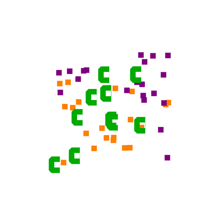
When the reaction starts there is only enzymes and substrate. As the reaction proceeds, the substrate is converted to products. The simulation below depicts the middle of an enzyme reaction where both reactants and products are present. The enzyme is represented by green shapes, the substrate is the purple squares and the products are the orange squares.
Out[]=
Below, is the equation for each of the states for any given enzyme. Free enzymes and substrates come together to form the Enzyme-Substrate-Complex (ESC) at a rate known as , also known as . In addition, the Enzyme-Substrate Complex can also be disassociated into the enzyme and substrate at the rate of or . Finally, the Enzyme-Substrate Complex can be converted into free enzyme and product at a rate known as .
k
+1
k
on
k
-1
k
off
k
cat
Out[]//DisplayForm=
E + S ESC E + P
k
+1
⇌
k
-1
k
cat
⟶
As a way to monitor the pace at which enzymes transform substrate into product, the Michaelis-Menten equation can be used. The Michaelis-Menten equation is a mathematical model describing enzyme kinetics. The Michaelis-Menten equation is based on the steady state assumption, which assumes that the rate of change (turnover rate) of substrate concentration in a multi-step reaction is constant. The Michaelis-Menten equation can be represent be the following:
v[S]+[S]
V
max
K
M
v represents the reaction rate of the particular enzyme. [S] represents the substrate concentration which influences the reaction rate. As substrate concentration increases, the reaction rate also increases, suggesting a directly proportional relationship. However, there is a maximum rate at which the enzyme itself can convert substrate into product. This means that even if you increase substrate concentration, the reaction rate will be saturated since the enzyme can’t increase its turnover rate of substrate into product. , which is the Michaelis-Menten constant, represents the substrate concentration at which the reaction rate is 50% of the . is also a measure of the affinity the enzyme has for the substrate. A lower value indicates a stronger affinity between enzyme and substrate, while a higher values indicates a weaker affinity. All these variables can be plotted on 3 main types of plots: the Lineweaver-Burk plot, the Eadie-Hofstee Plot, and the Hanes-Woolf plot.
k
m
V
max
k
m
k
m
k
m
Explanation of the Three Plots: Lineweaver Burk, Eadie-Hofstee, and Hanes-Woolf
Explanation of the Three Plots: Lineweaver Burk, Eadie-Hofstee, and Hanes-Woolf
To determine the different unknowns in the Michaels-Menten equation, visual representations can be used to help determine all the variables, given experimental data on the substrate concentrations and reaction rates. By utilizing graphing techniques, fitted lines can be applied to the data coordinates to evaluate and by examining different properties of the line such as x-intercept, y-intercept, and the slope.
k
m
V
max
The Lineweaver-Burk Plot
The Lineweaver-Burk Plot
The Lineweaver-Burk Plot is a common plot used in examining enzyme kinetics which is the inverse of the reaction rate plotted against the inverse of the substrate concentration. It is a linear model with the slope equal to /. Before the availability of computers, the Lineweaver-Burk plot was often used to compute the and . The y-intercept of the graph is the inverse of (1/) and and x-intercept of the graph represents -1/.
k
m
V
max
k
m
V
max
V
max
V
max
k
m
Derivation of the Lineweaver-Burk Equation
Derivation of the Lineweaver-Burk Equation
Michaels-Menten equation:v = +[S]Take the reciprocal of both sides:=+[S]Converting into slope intercept y = mx + b form:=×+
V
max[S]
K
m
1
v
K
m
V
max[S]
1
v
K
m
V
max
1
[S]
1
V
max
In[]:=

The Eadie-Hofstee Plot
The Eadie-Hofstee Plot
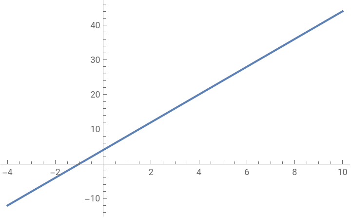
The Eadie-Hofstee Plot is another graphical representation of enzyme kinetics in which reaction rate is plotted as a function of the ratio between rate and substrate concentration. A plot of velocity against velocity over substrate concentration which yields as the y-intercept, / as the x-intercept, and as the negative slope.
V
max
V
max
k
m
k
m
Derivation of the Eadie-Hofstee Equation
Derivation of the Eadie-Hofstee Equation
Just like the Lineweaver-Burk equation, the Eadie-Hofstee equation is also derived from the main Michaelis-Menten equation:v = +[S]Take the reciprocal of both sides:=+[S]Multiply both sides by :=+[S]Multiply both sides by :=Distribute the V and simplify:=+VRearrange to isolate the V and convert the equation into slope-intercept form:V = -+
V
max[S]
K
m
1
v
K
m
V
max[S]
V
max
V
max
v
K
m
[S]
V
V
max
V(+[S])
K
m
[S]
V
max
VK
m
[S]
K
m
V
[S]
V
max
In[]:=

The Hanes-Woolf Plot
The Hanes-Woolf Plot
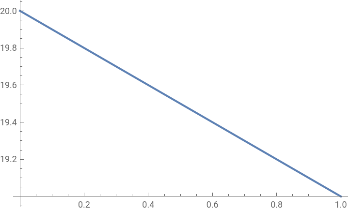
The Hanes-Woolf Plot is the final plot used to graph the Michaelis-Menten equation. Here, the ratio of substrate concentration to reaction rate is plotted against the substrate concentration. The x-intercept is -Km, the y-intercept is /, and the positive slope is 1/.
k
m
V
max
V
max
Derivation of the Hanes-Woolf Equation
Derivation of the Hanes-Woolf Equation
The Hanes-Woolf Plot is based on the equation for the Lineweaver-Burk plot. The first step to derive the Hanes-Woolf is to multiply substrate concentration on both sides of the Lineweaver-Burk equation:= +Re-arranging the variables, we get:=+ Converting into slope-intercept form, we get the final Hanes-Woolf equation:=[S]+
[S]
V
K
m
V
max
[S]
V
max
[S]
V
[S]
V
max
K
m
V
max
[S]
V
1
V
max
K
m
V
max
Example calculation to produce a Lineweaver-Burk plot from experimental data
Example calculation to produce a Lineweaver-Burk plot from experimental data
Once experimental data is obtained from a laboratory, here is how one would go about trying to make a Lineweaver-Burk Plot from the raw data collected:
1. Format the data of substrate concentration and reaction rate into (x,y) coordinates to get a list of lists and make element a Quantity object with the numerical value and the units separated like demonstrated below:
1. Format the data of substrate concentration and reaction rate into (x,y) coordinates to get a list of lists and make element a Quantity object with the numerical value and the units separated like demonstrated below:
Enter the data:
2. When plotting the graph in the future, we can only plot raw numerical values, so we need to apply the QuantityMagnitude function to remove the units
Extract magnitudes of measured data:
3. Since we are graphing a Lineweaver-Burk plot, we have to take the reciprocal of both the substrate concentration and reaction rate
Take the reciprocals of the plot data:
4. Now we plot these points on the Lineweaver Burk graph
Display a scatter plot:
5. From the data points on the graph, we now have to create a line of best fit using the LinearModelFit function to see where the x and y-intercepts are
Compute a linear approximation:
Show the result:
The process of extracting, rearranging , finding Linear Model Fits, and graphing data can be quite tedious and wouldn’t it be better if there was a function to this! The process of building the Michaels-Menten function is illustrated below.
Data Processing
Data Processing
The data the Michaelis Menten function processes experimental substrate concentration and reaction rate data pairs with units of Molar for the substrate concentration and Molar/Minute for the reaction rate. If the user inputs data as invalid, that doesn’t match the format that this function takes as a parameter, the function returns $Failed.
To process the data before being evaluated, MatchQ is used to test if the Data is a list of lists (x,y) coordinates and if all the elements in the list are quantity objects:
If the data inputted is not in Molar and Molar/Minutes for the (x,y) pairs respectively, the function QuantityMagnitude is applied to all the elements in the list to be converted to Molar and Molar/Minute and also to retrieve raw number data so computation on them is possible. Hence, the substrate concentrations can be accepts concentration in any molarity. Likewise, reaction rates can be in any amount concentration unit per time unit.
The following code extracts the x-coordinates and y-coordinates independently from the data after being processed:
Extracting and Fitting Data
Extracting and Fitting Data
Each of different plots consists of manipulated x and y-coordinates to match the axis on their respective graphs.
The Transpose function is used to pair the x and y-values back into (x,y) coordinate form:
Here, all the x-values from each of the transformed data sets is taken to set the Plot Range which graphing each type of data:
Do the fits:
Compute values:
Creating Plots and Associations
Creating Plots and Associations
This is the association for the Lineweaver Burk Plot. The Normal function on “fit” gives the raw linear equation. The minimum x-value that needs to be displayed for this plot is the x-intercept or the -1/km as represented on the graph. The maximum x-value displayed would be the max number from the x-value coordinates. The axes were also labeled 1/Molar and Minutes/Molar respectively. The slope and variance were also calculated. The Show function was used to display both the data coordinates and the line of best fit.
Lineweaver-Burk data association:
I used a similar process for the Eadie-Hofstee plot where the minimum x-value for the Plot Range was 0 while the max was the maximum of all the x-values. The Axes were labeled Molar/Minutes and 1/Minutes on the x and y axes respectively.
Eadie-Hofstee data association:
Finally, was the Hanes-Woolf plot in which the minimum x-value was -1/Km and the maximum was the max of all the x-values present. The x-axis was plotted on Molar units while the y-axis was plotted on Molar^2/Minutes Units. Just like before, both slope and variance were calculated.
Hanes-Woolf data association:
Michaels-Menten Function
Michaels-Menten Function
Here are all the pieces of function fitted together with example test data:
Define the function:
Now let’s dig deeper into the output for each plot type.
Lineweaver-Burk plot:
Eadie-Hofstee plot:
Hanes-Woolf plot:
Discussion
Discussion
The Eadie-Hofstee Plot is thought to be more robust against error-prone data than the Lineweaver-Burk plot, particular since its equal weight-age to the data points any range of substrate concentration and reaction rate while the Lineweaver-Burk unevenly weights these data points. However, one drawback from the Eadie-Hofstee plot is that both the x and y-axis (independent variables) are dependent on the reaction rate. Hence, any experimental error present will affect both axes.
The Hanes-Woolf Plot is considered the most accurate for kinetic parameters of the three. However, its major drawback is that neither the x and y-values represents independent values and that they are both dependent on the substrate concentration.
Conclusion
Conclusion
This function demonstrated a method in which experimental enzyme kinetics data can be analyzed as well as an exploration into how different interpretations of the data can provide unique statistical viewpoints. The Michaelis-Menten equation is used widely in medicinal chemistry such as determining if drugs or vaccines are effective in treating diseases. Through a complete data evaluation, this function can provide a thorough overview of the kinetic parameters of the enzymes serving as a powerful and important computational tool in the future
Future Work
Future Work
Acknowledgements
Acknowledgements
I would like to take my mentor Jason Sonnenberg, the TA’s who introduced me to the idea of computational enzyme kinetics and Maggie Wear for discussing with me its important relevance in medicinal chemistry.
References
References
“Biochemistry | Michaelis Menten Equation.” YouTube, 26 April 2017, http://youtube.com/watch?v=4eLjRcHnMCk. Accessed 13 July 2023.
“Enzyme Kinetics in Medicinal Chemistry.” PharmaFactz, https://pharmafactz.com/medicinal-chemistry-understanding-enzyme-kinetics/. Accessed 13 July 2023.
“Hill Equation - Interactive Graph.” PhysiologyWeb, 22 October 2014, https://www.physiologyweb.com/calculators/hill_equation_interactive_graph.html. Accessed 13 July 2023.
Nelson, David L, and Michael M Cox. Lehninger Principles of Biochemistry. 4th ed., W. H. Freeman, 2004.
“10.2: The Equations of Enzyme Kinetics.” Chemistry LibreTexts, 1 September 2020, https://chem.libretexts.org/Bookshelves/Physical_and_Theoretical_Chemistry_Textbook_Maps/Map%3A_Physical_Chemistry_for_the_Biosciences_(Chang)/10%3A_Enzyme_Kinetics/10.02%3A_The_Equations_of_Enzyme_Kinetics. Accessed 13 July 2023.
CITE THIS NOTEBOOK
CITE THIS NOTEBOOK
Build a function for biochemical enzyme kinetics
By Srijith Rangan
Wolfram Community, STAFF PICKS, July 13, 2023
https://community.wolfram.com/groups/-/m/t/2965033
By Srijith Rangan
Wolfram Community, STAFF PICKS, July 13, 2023
https://community.wolfram.com/groups/-/m/t/2965033