Before we start polygons, here is some info on an important example that we will use eventually.
Table[{i,2^i,Sum[1./n,{n,1,2^i}],1.+i/2},{i,1,20}]//MatrixForm
Here is Mathematica code for generating shaded polygons. The variable is the number of sides of the polygon, and theta is the angle of rotation. It's set up so you change the fraction, the portion of a circle you want to rotate. The midpoint figures are generated by using as your fraction, where is the number of sides. See the examples below. FYI: The area of a regular polygon with n sides and side length s is So, if you have a pentagon with side length 1, the area is
n
1/(2n)
n
a=ncot(π/n).
1
4
2
s
In[]:=
(1/4)(5)(1^2)Cot[Pi/5]
Out[]=
5
4
1+
2
5
In[]:=
N[%]
Out[]=
1.72048
The variable n is the number of sides in your polygon, while theta is the angle of rotation. If you make the fraction greater than 1/(2n), you’re rotating past the midpoint of the first side and you could get an equivalent picture with a smaller angle of rotation.
In[]:=
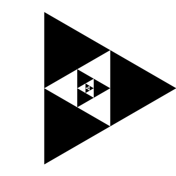
n=3.;theta=2Pi(1/6);(*Idonotrecommendchangingthecodebelowthispoint*)endval=500;r=1;t0=0.;alpha=Pi(1-2./n);phi=2.Pi/n-theta;s=Sqrt[(rCos[t0]-rCos[t0+2Pi/n])^2+(rSin[t0]-rSin[t0+2Pi/n])^2];m=Sin[alpha]/(Sin[phi]+Sin[theta]);wholearea=1/4nsCot[Pi/n];showlist={};obj=Polygon[Table[{rCos[t0+2Pii/n],rSin[t0+2Pii/n]},{i,1,n}]];showlist=AppendTo[showlist,{GrayLevel[0],obj}];Do[t0=t0+theta;s=ms;y=sSin[theta]/Sin[alpha];r=Sqrt[r^2+y^2-2ryCos[alpha/2]];obj=Polygon[Table[{rCos[t0+2Pii/n],rSin[t0+2Pii/n]},{i,1,n}]];showlist=AppendTo[showlist,{GrayLevel[Mod[j,2]],obj}],{j,1,endval}];area=Sum[(-1)^nm^(2n),{n,0,Infinity}];Print[wholearea," ",area," ",area/wholearea];Show[Graphics[showlist],AspectRatioAutomatic,PlotRange{{-1,1},{-1,1}}]
0.75 0.8 1.06667
Out[]=
Area Computer:
n=3;theta=2Pi/10;alpha=Pi(1-2./n);phi=2.Pi/n-theta;m=Sin[alpha]/(Sin[phi]+Sin[theta]);Sum[(-1)^nm^(2n),{n,0,Infinity}]
In[]:=
n=7.;theta=2Pi(1/20);(*Idonotrecommendchangingthecodebelowthispoint*)endval=500;r=1;t0=0.;alpha=Pi(1-2./n);phi=2.Pi/n-theta;s=Sqrt[(rCos[t0]-rCos[t0+2Pi/n])^2+(rSin[t0]-rSin[t0+2Pi/n])^2];m=Sin[alpha]/(Sin[phi]+Sin[theta]);showlist={};obj=Polygon[Table[{rCos[t0+2Pii/n],rSin[t0+2Pii/n]},{i,1,n}]];showlist=AppendTo[showlist,{GrayLevel[0],obj}];Do[t0=t0+theta;s=ms;y=sSin[theta]/Sin[alpha];r=Sqrt[r^2+y^2-2ryCos[alpha/2]];obj=Polygon[Table[{rCos[t0+2Pii/n],rSin[t0+2Pii/n]},{i,1,n}]];showlist=AppendTo[showlist,{GrayLevel[Mod[j,2]],obj}],{j,1,endval}];Show[Graphics[showlist],AspectRatioAutomatic,PlotRange{{-1,1},{-1,1}}]
Out[]=
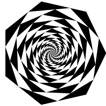
n=4.;theta=2Pi(1/60);(*Idonotrecommendchangingthecodebelowthispoint*)endval=500;r=1;t0=0.;alpha=Pi(1-2./n);phi=2.Pi/n-theta;s=Sqrt[(rCos[t0]-rCos[t0+2Pi/n])^2+(rSin[t0]-rSin[t0+2Pi/n])^2];m=Sin[alpha]/(Sin[phi]+Sin[theta]);showlist={};obj=Polygon[Table[{rCos[t0+2Pii/n],rSin[t0+2Pii/n]},{i,1,n}]];showlist=AppendTo[showlist,{GrayLevel[0],obj}];Do[t0=t0+theta;s=ms;y=sSin[theta]/Sin[alpha];r=Sqrt[r^2+y^2-2ryCos[alpha/2]];obj=Polygon[Table[{rCos[t0+2Pii/n],rSin[t0+2Pii/n]},{i,1,n}]];showlist=AppendTo[showlist,{GrayLevel[Mod[j,2]],obj}],{j,1,endval}];Show[Graphics[showlist],AspectRatioAutomatic,PlotRange{{-1,1},{-1,1}}]

I've also introduced color, just for fun. The code is below, and I've included a few of my favorites. The color is controlled through the redscale, bluescale and greenscale variables, together with the redfunct, greenfunct, and bluefunct functions.