The Weierstrass elliptic function is just about the simplest possible elliptic function, which means it is a doubly-periodic meromorphic function on the complex plane .
℘
A function being doubly-periodic means that there exist ,∈ with ∉ so that and for all . More generally, this means that for any , and so the behavior of is completely determined by what it does on the fundamental domain which is (any translate of) the parallelogram with corners at . Indeed, if is the lattice determined by , then we can just as well think of as a function on the quotient space , which a topologist or differential geometer would probably call a torus and a number theorist or algebraic geometer would probably call an elliptic curve. This is the source of the name elliptic function.
f
ω
1
ω
2
ω
1
ω
2
f(z+)=f(z)
ω
1
f(z+)=f(z)
ω
2
z∈
f(z+m+n)=f(z)
ω
1
ω
2
m,n∈
f
0,,,+
ω
1
ω
2
ω
1
ω
2
Λ={m+n:m,n∈}
ω
1
ω
2
(,)
ω
1
ω
2
f
/Λ
If a doubly-periodic function is entire, then it must in particular be continuous and hence bounded on the fundamental domain, and therefore on the entire plane, so Liouville's theorem implies that it must be constant. Therefore, any non-constant doubly-periodic function must have singularities, and the ones with only isolated poles (i.e., the meromorphic ones) are the elliptic functions.
f
Let be the boundary of the fundamental domain of an elliptic function , oriented clockwise. Then , where the first equality follows from double-periodicity (since the values on opposite sides of the fundamental domain are the same, but traversed in opposite directions) and the second equality is the residue theorem (here the sum is over all poles in the fundamental domain). Since the sum of residues can’t be zero if has a single simple pole, this proves:
γ
f
0=f=f(z)
∮
γ
n
∑
k=1
Res
z=
z
k
f
Theorem. Any elliptic function has at least 2 poles (counting multiplicity) in its fundamental domain.
If you try to build an elliptic function with a single pole of order 2 at the origin (and hence also at all the lattice points) and so that the leading term in the Laurent series at the origin is , you end up with the Weierstrass function .
1
2
z
℘(z):=+-
1
2
z
∑
ω∈Λ\{0}
1
2
(z-ω)
1
2
ω
(This is explained very well in sections 1.5–1.6 of Apostol’s Modular Functions and Dirichlet Series in Number Theory.)
Of course, depends on the periods and (or equivalently on the lattice ), so it is sometimes helpful to indicate it by .
℘
ω
1
ω
2
Λ
℘(z;,)
ω
1
ω
2
As in Mathematica’s definition WeierstrassP[z, , it is also common to write , where the invariants and are functions of (or really of ) that show up as coefficients in the Laurent series of and also in the differential equation .
{,}]
g
2
g
3
℘(z;,)
g
2
g
3
g
2
g
3
(,)
ω
1
ω
2
τ=
ω
2
ω
1
℘
℘'=4-℘(z)-
2
(z)
3
℘(z)
g
2
g
3
In any case, Mathematica can easily convert between (half-)periods and invariants using WeierstrassInvariants and WeierstrassHalfPeriods.
Here’s a visualization of on the square lattice using domain coloring, which shows phase as hue and modulus as brightness:
℘
In[]:=
Module[{g2,g3},{g2,g3}=WeierstrassInvariants[{1/2,I/2}];Show[ComplexPlot[WeierstrassP[z,{g2,g3}],{z,-2-2I,2+2I},PlotRangePaddingNone,BoundaryStyleNone],Graphics[{Thickness[.005],Table[InfiniteLine[{{0,n},{1,n}}],{n,-5,5}],Table[InfiniteLine[{{n,0},{n,1}}],{n,-5,5}]}],PlotRange->2,ImageSize->Large]]
Out[]=
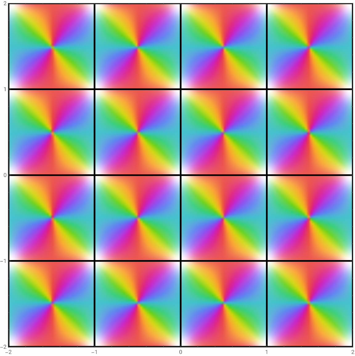
We can clearly see a double pole at the lattice points (since the colors appear twice in clockwise order) and a double zero in the center of the fundamental domain (again, colors appear twice, but now in counterclockwise order).
And here’s the Weierstrass function for the 60º rhombus:
In[]:=
Module{g2,g3},{g2,g3}=NWeierstrassInvariants,;ShowComplexPlot[WeierstrassP[z,{g2,g3}],{z,-2-2I,2+2I},PlotRangePaddingNone,BoundaryStyleNone],GraphicsThickness[.005],TableInfiniteLine0,n,1,n,{n,-5,5},TableInfiniteLine{n,0},12+n,,{n,-5,5},PlotRange->2,ImageSize->Large
1
2
Iπ/3
E
2
3
2
3
2
3
2
Out[]=
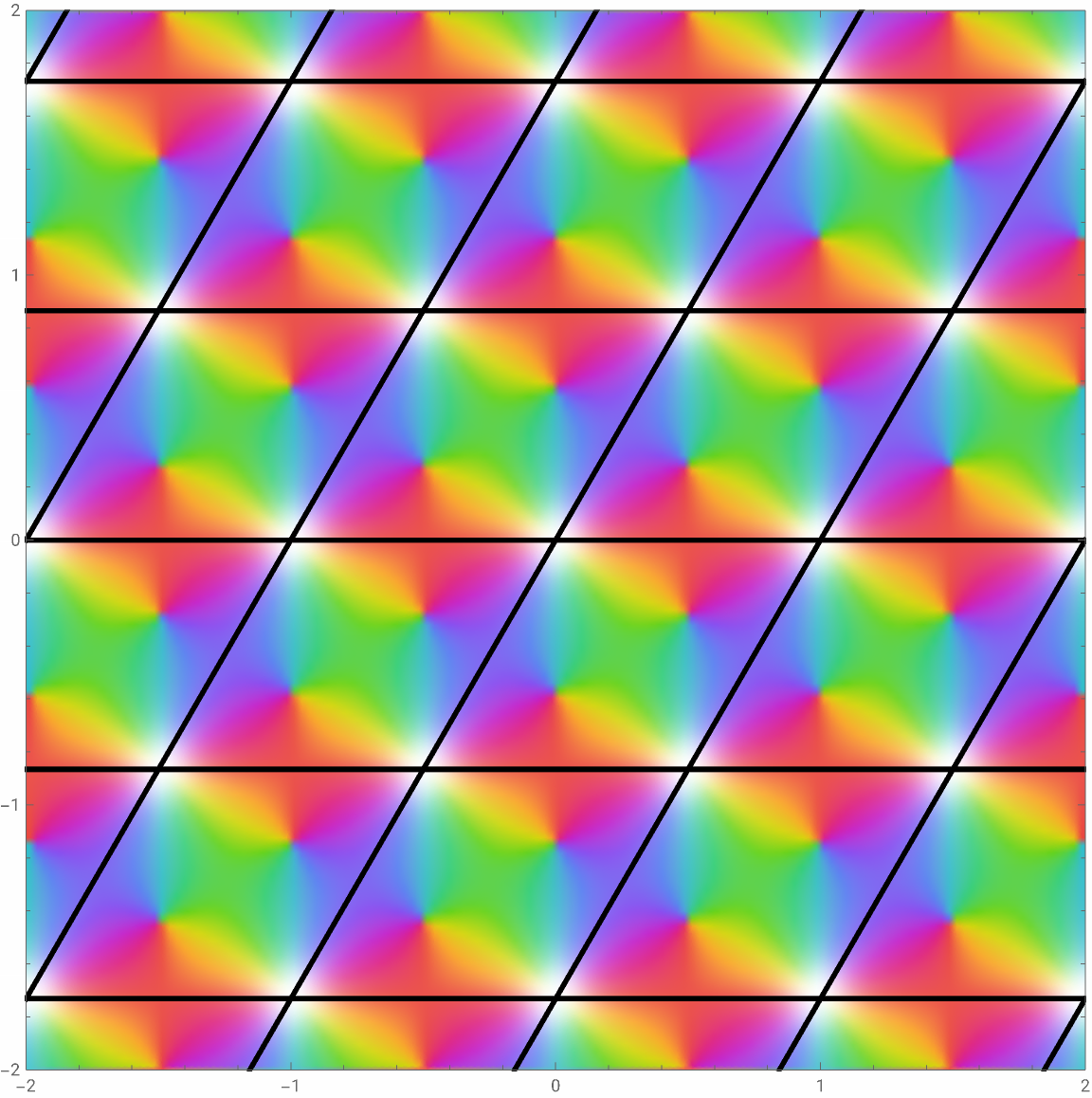
Notice that we still have the double pole, but the double zero has now split into two simple zeros.
To get a looping animation out of domain coloring plots of Weierstrass functions, one strategy is to find a periodic path in the space of lattices. We can do that using the modular flow, which I previously used to produce this animation.
The idea is to let be the lattice of points of the form , where and is an integer point in the plane.
Λ
P
x |
y |
P=
-1 | - 2 |
1 | - 2 |
∈
x |
y |
2
In[]:=
P=-1,-
2
,1,-2
;Here’s a picture of :
Λ
In[]:=
Graphics[{Thickness[.005],PointSize[Large],Table[Point[P.{x,y}],{x,-10,10},{y,-10,10}]},PlotRange->8]
Out[]=
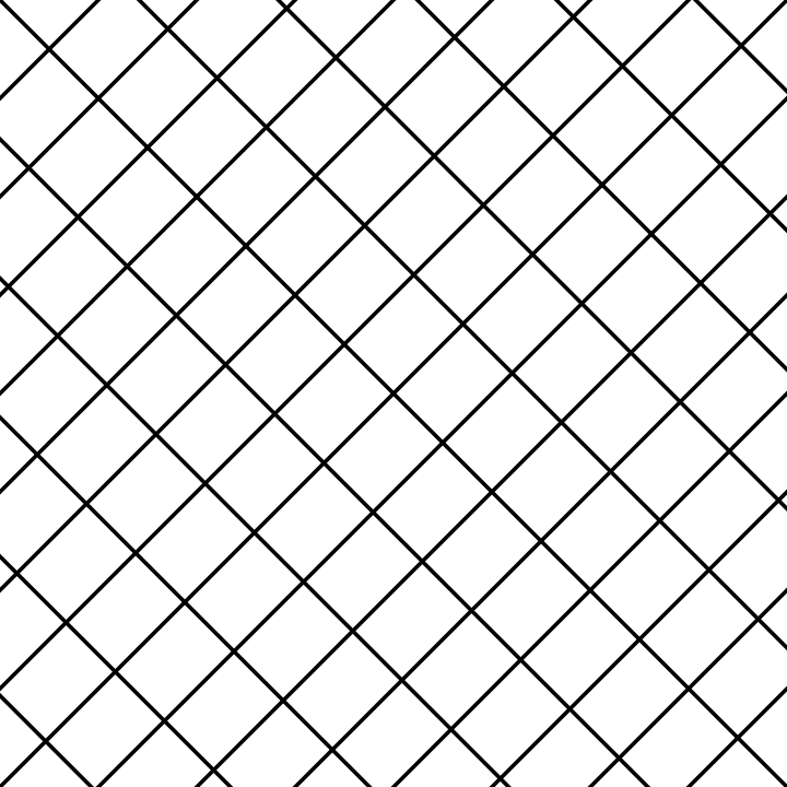
And the corresponding tiling by copies of the fundamental domain:
In[]:=
Graphics[{Thickness[.005],Table[InfiniteLine[{P.{0,y},P.{1,y}}],{y,-10,10}],Table[InfiniteLine[{P.{x,0},P.{x,1}}],{x,-10,10}]},PlotRange->8]
Out[]=
And build the frames of the animation (note that we’re rotating the color palette a quarter turn):
Which we can export to a GIF:
Or visualize directly using ListAnimate:
CITE THIS NOTEBOOK
CITE THIS NOTEBOOK
Phase (periodic family of Weierstrass functions)
by Clayton Shonkwiler
Wolfram Community, STAFF PICKS, May 22, 2025
https://community.wolfram.com/groups/-/m/t/3465926
by Clayton Shonkwiler
Wolfram Community, STAFF PICKS, May 22, 2025
https://community.wolfram.com/groups/-/m/t/3465926