ABSTRACT (original article): We consider a multitype Galton-Watson process that allows for the mutation and reversion of individual types in discrete and continuous time. In this setting, we explicitly compute the time evolution of quantities such as the mean and distributions of different types. This allows us in particular to estimate the proportions of different types in the long run, as well as the distribution of the first time of occurrence of a given type as the tree size or time increases. Our approach relies on the recursive computation of the joint distribution of types conditionally to the value of the total progeny. In comparison with the literature on related multitype models, we do not rely on approximations. CITATION (original article): Huang, Q., & Privault, N. (2026). Binary Galton–Watson trees with mutations. Communications in Nonlinear Science and Numerical Simulation, 156, 109623. https://doi.org/10.1016/j.cnsns.2025.109623
Multitype Galton–Watson processes are used in population genetics and evolutionary biology to model the propagation and extinction of mutant types. Here, we consider a multitype Galton–Watson process that allows for the mutation and reversion of individual types in discrete and continuous time.
More precisely, we consider multitype random binary trees in which every node bears an integer type 𝑗 ≥ 0 and may generate either no offspring, or two offsprings, one with type 0 and one with type 𝑗 + 1.
Our analysis covers both the discrete-time case, in which two offsprings are generated with probability 𝑝 ∈ (0, 1) and no offspring is generated with probability 𝑞 := 1 − 𝑝, and the continuous-time setting, which yields a multitype Galton—Watson process.
In this setting, we explicitly compute the time evolution of quantities such as the mean and distributions of different types. This allows us in particular to estimate the proportions of different types in the long run, as well as the distribution of the first time of occurrence of a given type as the tree size or time increases. Our approach relies on the recursive computation of the joint distribution of types conditionally to the value of the total progeny.
Reference: Binary Galton–Watson trees with mutations.
doi: https://doi.org/10.1016/j.cnsns.2025.109623
doi: https://doi.org/10.1016/j.cnsns.2025.109623
Discrete-time case
Discrete-time case
In[]:=
ClearAll["Global`*"]
In[]:=
Quiet[Needs["Combinatorica`"]]
In[]:=
catalan[n_]:=Binomial[2*n,n]/(n+1)
The next code block implements the recursive calculation of Theorem 2.2.
In[]:=
b[j_,m__]:=b[j,m]=(Module[{i,k,l,n,mk,mm,m2,sum},n=Length[m];If[n==0,Return[1]];If[m[[n]]==0,Return[b[j,Drop[m,-1]]]];sum=0;m2=Append[m,0];Do[If[m2[[j+l]]>m2[[j+l+1]],mk={};Do[mk=Append[mk,Compositions[m2[[i]]-Boole[j<i<=j+l],l]],{i,1,n}];Do[If[AllTrue[Reverse/@Transpose[mm],OrderedQ],sum=sum+Product[b[0,Transpose[mm][[k]]],{k,1,l}]],{mm,Tuples[mk]}]],{l,1,n-j}];Return[sum]])
The next code block implements the calculation of the conditional mean (2.7) using Theorem 2.2.
In[]:=
CondMeanRecursive[j_,m_,l_]:=CondMeanRecursive[j,m,l]=(Module[{i,mm,n,sum},sum=0;If[j==0,Do[Do[If[Last[mm]>=1&&OrderedQ[Reverse[mm[[1;;n]]]],sum=sum+b[0,mm]*mm[[l]]/catalan[m]],{mm,Compositions[m,n]}],{n,Max[l,1],m}],n=j;Do[If[Total[mm[[1;;n]]]==0,sum=sum+b[j,mm]*mm[[l]]/catalan[m]],{mm,Compositions[m,n]}];Do[Do[If[Last[mm]>=1&&mm[[j]]+1>=mm[[j+1]]&&OrderedQ[Reverse[mm[[1;;j]]]]&&OrderedQ[Reverse[mm[[j+1;;n]]]],sum=sum+b[j,mm]*mm[[l]]/catalan[m]],{mm,Compositions[m,n]}],{n,Max[l,j+1],m+j}]];Return[N[sum]]])
The next code block implements the calculation of the conditional mean (2.7) in Corollary 2.3.
In[]:=
CondMeanNonRecursive[j_,m_,l_]:=(Boole[0<l-j<=m]*(l-j+1)/(m+1)*Binomial[2*m-l+j,m]/catalan[m]+Boole[m>=l]*Binomial[2*m-l,m+1]/catalan[m])
The next two code blocks implement the Monte Carlo computation of the conditional mean (2.7).
In[]:=
SampleTree[c_,l_,c2_,p_]:=(Module[{add1,add2,cc2,U},cc2=c2;If[c==l,cc2+=1];U=RandomVariate[UniformDistribution[1]][[1]];If[U<p,add1=SampleTree[0,l,0,p];add2=SampleTree[c+1,l,0,p];Return[{1+add1[[1]]+add2[[1]],cc2+add1[[2]]+add2[[2]]}],Return[{0,cc2}]]])
In[]:=
CondMeanMonteCarlo[j_,k_,l_,p_]:=(temp=0;c4=0;If[j==l,c5=-1,c5=0];For[i=1,i<=1000000,i++,sample=SampleTree[j,l,c5,p];If[sample[[1]]==k,c4+=1;temp=temp+sample[[2]]]];Return[N[temp/c4]])
Next, we check the numerical consistency of all three above algorithms (recursive, non-recursive, Monte Carlo).
In[]:=
j=1;m=5;l=3;CondMeanRecursive[j,m,l]
Out[]=
0.833333
In[]:=
N[CondMeanNonRecursive[j,m,l]]
Out[]=
0.833333
In[]:=
j=1;m=5;l=3;p=0.4;CondMeanMonteCarlo[j,m,l,p]
Out[]=
0.833873
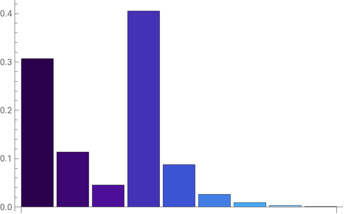
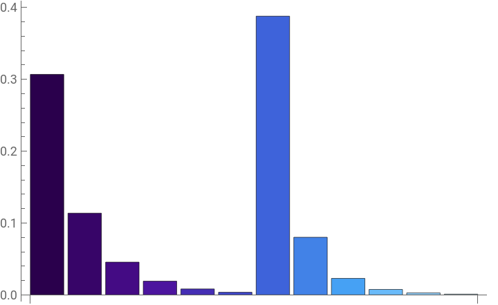
The next code plots the limiting proportions (2.11).
In[]:=
LimitingProportions[j_,l_,p_]:=(If[l<=j,Beta[p,1+l,-1]*(1-p)/p,Beta[p,1+l,-1]*(1-p)/p+((l+1-j)*Beta[p,l-j,0]-p^(l-j)/(1-p))*(1-p)/p])
In[]:=
jj=3;BarChart[Table[LimitingProportions[jj,l,1/2],{l,1,3*jj}],ChartStyle->{"DeepSeaColors"}]
Out[]=
In[]:=
jj=6;BarChart[Table[LimitingProportions[jj,l,1/2],{l,1,2*jj}],ChartStyle->{"DeepSeaColors"}]
Out[]=
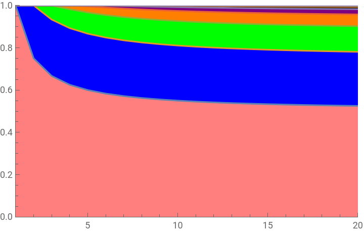
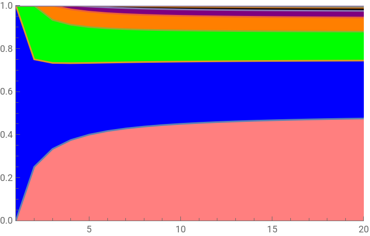
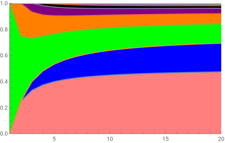
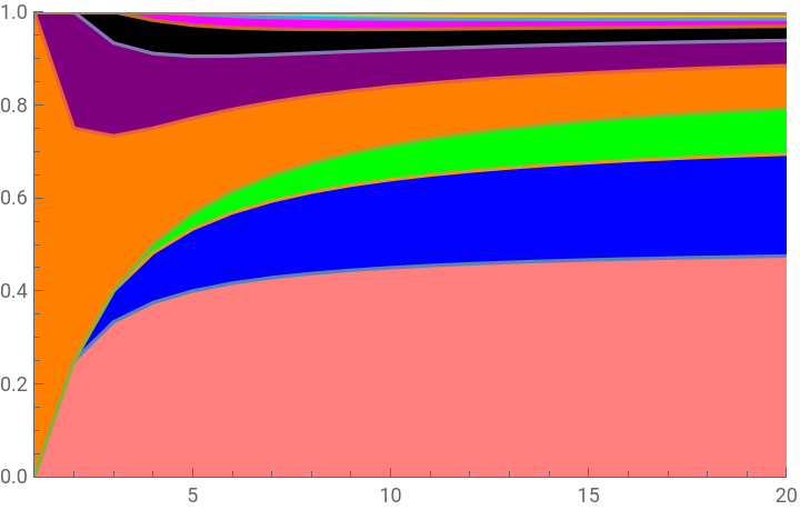
The next code is plotting the conditional average type proportions in (2.7) in Figure 2 as an application of Corollary 2.3.
In[]:=
R=20;S=20;A=ConstantArray[ConstantArray[ConstantArray[0,R],S],S+1];
In[]:=
colors=<|0->Pink,1->Blue,2->Green,3->Orange,4->Purple,5->Black,6->Magenta,7->Cyan,8->Orange,9->Purple|>;
In[]:=
For[j=0,j<=3,j++,Do[Do[A[[j+1]][[l]][[m]]=CondMeanNonRecursive[j,m,l]/m,{m,1,R}],{l,1,S}];dataNorm=Accumulate[#]&/@Transpose@A[[j+1]];Print["j=",j];ListPlot[Transpose@Reverse[Reverse@dataNorm],Joined->True,Filling->Table[i->{{i-1}/.{0}->0,colors[Mod[i-1,10]]},{i,S}],PlotRange->{{1,R},{0,1}}]//Print]
j=0
j=1
j=2
j=3
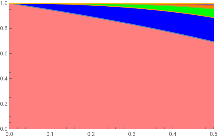
The next code is plotting the average type proportions (2.10) in Figure 3 as an application of Corollary 2.4.
In[]:=
S=8;For[j=0,j<=5,j++,B={};Do[B=Append[B,f[pp_]=LimitingProportions[j,l,pp]],{l,1,S}];dataNorm=Accumulate[B];Print["j=",j];Plot[dataNorm,{pp,0,1/2},Filling->Table[i->{{i-1}/.{0}->0,colors[Mod[i-1,10]]},{i,S}],PlotRange->{{0,1/2},{0,1}}]//Print]
j=0
Continuous-time case
Continuous-time case
The next code block implements the recursive calculation of Theorem 3.2.
The next code block implements the calculation of the conditional mean (3.7) using Theorem 3.2.
The next code block implements the calculation of the extinction probability (3.9) using Theorem 3.2
The next code blocks implement the Monte Carlo computation of the extinction probability (3.9).
The next code is plotting the expected counts (3.6) in Figure 6 as an application of Theorem 3.2.
The next code is plotting the tails CDFs and PDFs (3.8) in Figures 7 and 8 as an application of Theorem 3.2.
The next code is plotting the mean proportions of types (3.10) in Figure 9 as an application of Theorem 3.2.
CITE THIS NOTEBOOK
CITE THIS NOTEBOOK
Binary Galton-Watson trees with mutations
by Qiao Huang & Nicolas Privault
Wolfram Community, STAFF PICKS, January 21, 2026
https://community.wolfram.com/groups/-/m/t/3618886
by Qiao Huang & Nicolas Privault
Wolfram Community, STAFF PICKS, January 21, 2026
https://community.wolfram.com/groups/-/m/t/3618886