Computational Modeling
for Complex Systems
Computational Modeling
for Complex Systems
for Complex Systems
Phileas Dazeley-Gaist, Wolfram Research
Indiana University, October 2025
Indiana University, October 2025
1. Getting Started With wolfram Language
1. Getting Started With wolfram Language
Getting set up: Installing Wolfram at Indiana University
Getting set up: Installing Wolfram at Indiana University
1
.Head to www.wolfram.com/siteinfo
2
.Enter your IU email address in the input field
3
.Download and install the Wolfram App
4
.Create a Wolfram account with your institutional email address,
5
.Log into the Wolfram app using your account
Wolfram Language ABCs
Wolfram Language ABCs
Before we get into modeling techniques with Wolfram Language, here are a few keys you’ll need to understand how to read Wolfram Language code.
A few warnings before we jump in:
Wolfram Language is not a programming language you ever fully learn. It’s just too big.
Don’t panic if you don’t immediately understand something. Programming always looks a little mysterious until you try it out, but it’s really not too bad.

I’ll send you this notebook later, so you’ll be able to review all the code, copy and paste examples, and mess about with it on your own time.
Please feel free to jump in to ask me questions. I’ll also take questions at the end of the talk.
Symbolic Expressions
Symbolic Expressions
1
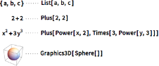
.Wolfram Language is a symbolic programming language. Everything in Wolfram Language (with very few exceptions such as real numbers and integers) is a symbolic expression.
2
.All symbolic expressions have the same fundamental structure: head[arguments].
For example:
For example:
a+b
In[]:=
FullForm[a+b]
Out[]//FullForm=
Plus[a,b]
Variable Assignment and Function Definitions
Variable Assignment and Function Definitions
Variable assignments allow you to define things by name and refer to them later.
There are two types of variable assignment in WL: , and
Set (=)
Set (=)
Set: sets the symbol to the value .
var=val
var
val

Variable assignment using Set:
In[]:=
a=1;
Fetch the value of :
a
In[]:=
a
Out[]=
1
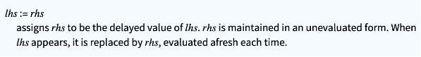
SetDelayed (:=)
SetDelayed (:=)
SetDelayed: sets the symbol to the unevaluated from of . Whenever is requested, is evaluated and then returned.
var:=val
var
val
var
val
Delayed variable assignment using SetDelayed:
In[]:=
randomLetter:=RandomChoice[Alphabet[]]
Fetch the value of 3 times:
randomLetter
In[]:=
{randomLetter,randomLetter,randomLetter}
Out[]=
{z,r,w}
ClearAll
ClearAll
Make the Wolfram Kernel forget a definition using ClearAll:
In[]:=
ClearAll[a]
The symbol is now blue, which tells us it is undefined. Evaluating just returns the symbol :
a
a
a
In[]:=
a
Out[]=
a
ClearAll is an example of a built-in Wolfram Language function.
Function definitions
Function definitions
Functions are definitions for procedures. They are templates that take inputs (called arguments) and perform some action based on the provided information.
Define a function:
In[]:=
f[arg_(*←apatternnamedarg*)]:=Highlighted[arg,Background->StandardGreen]
Evaluate the function using the syntax :
function[,…,]
arg
1
arg
n
In[]:=
f["elephant"]
Clear the function definition:
In[]:=
ClearAll[f]
Pure (Anonymous) Functions
Pure (Anonymous) Functions
The Wolfram Language allows what it calls pure functions, indicated by ending with Their first argument is indicated by .
Pure functions are also known as anonymous functions or lambda expressions.
Make a pure function for adding 1:
In[]:=
(#+1)&
Out[]=
#1+1&
If a pure function is given as the head of an expression, the function is applied to the arguments:
In[]:=
(#+1)&[50]
Out[]=
51
Here is a function of several arguments:
{#2,1+#1,#1+#2}&
Out[]=
{#2,1+#1,#1+#2}
In[]:=
{#2,1+#1,#1+#2}&[a,b]
Out[]=
{b,1+a,a+b}
Importing data into a Wolfram Notebook
Importing data into a Wolfram Notebook
There are a few ways to import data into Wolfram notebooks:
Copying and pasting into the notebook directly
Dragging and dropping files and images into a notebook
Using the function
Here’s a short overview of how the Import function works:
In[]:=
?Import
Out[]=
Import a picture:
In this case, the file format is inferred from the file extension.
Import some data from a file:
Here, the second argument specifically tells the function to interpret the data as a Tabular object.
The Import function supports many import formats:
Storing data (List, Association, Dataset, and Tabular)
Storing data (List, Association, Dataset, and Tabular)
Let’s walk through a few of the most common ways of storing data in Wolfram Language: lists, associations, datasets, and tabular objects:
Lists
Lists
Lists take the form {element1, element2,…} and can contain arbitrary elements.
Define a list:
You can retrieve an element from a list using “part” notation:
Associations
Associations
Associations are like lists, but they link values to names called keys.
Define an association:
You can retrieve elements from an association using a specific key:
You can also retrieve an element from an association using “part” notation:
Datasets
Datasets
Datasets are a nice way of representing structured data based on a hierarchy of lists and associations.
For example, we can make a dataset from the association we just defined above:
If we have a list of associations with the same keys, it will make a table:
Tabular objects
Tabular objects
Tabular objects are more data-efficient representations of tabular data. They can store huge datasets and perform complex operations on them fast.
You can make a tabular object out of any tabular Dataset object:
Or you can import external tables as Tabular objects:
For more information about Tabular objects, I recommend these guide pages from the Wolfram Documentation:
2. Complex Systems and System Models
2. Complex Systems and System Models
What are Complex Systems?
Questions to get us going
Questions to get us going
How do ecosystems sustain themselves and evolve?
Why does biodiversity tend to increase with ecological succession?
What processes allow ants to organise and act collectively as a single intelligent and self-sustaining unit?
How do microeconomic interactions between economic agents give rise to the global economy?
Working Definition
Working Definition
Complex systems are systems composed of many interacting parts, in which the local interaction between the parts result in global emergent phenomena.
Complex Systems exhibit a gestalt, or “more than the sum of the parts” behaviour.
Complex Systems Modeling Approaches
Modeling real world phenomena can be approached in a huge variety of ways.
Here are some common dimensions and classes of model to consider in your modeling journey:
Dimensions of modelling
Dimensions of modelling
(This is a non-exhaustive list)
Discrete Continuous (States, Variables)
Stochastic Deterministic (Processes, Mechanisms)
Static Dynamic (Do the modeled phenomena evolve in time?)
Microscopic Macroscopic (individual entities vs. collective variables, e.g. agent vs. populations)
Open Closed (Exchange with environment vs. isolated)
Memoryless Path-dependent (See Markovian vs. non-Markovian processes.)
Common model types
Common model types
Classical models: Ordinary and partial differential equations.
System models and compartmental models
Agent based models (ABMs)
Markov chains and stochastic processes
Network models
Cellular automata
Statistical and data driven models (e.g. machine learning techniques)
Model validation
Model validation
Frequent model validation approaches
Frequent model validation approaches
Qualitative validation: Does the model reproduce known qualitative behaviors and patterns?
Quantitative validation: How well do model outputs match empirical data?
Statistical comparison with observations
Fitting parameters to experimental data
Predictive accuracy on held-out data
Sensitivity analysis: How robust are model predictions to parameter variations?
Mechanistic validation: Are the underlying mechanisms realistic and well-justified?
Theoretical grounding
Consistency with domain knowledge
Common challenges
Common challenges
Data limitations:
Insufficient or noisy data for validation
Scale mismatch: Models at one scale (e.g., microscopic) may be hard to validate against data at another (e.g., macroscopic)
Parameter identifiability and multiple-realisability: Multiple parameter sets may produce similar outputs, just as multiple sets of causes can lead to similar consequences.
Computational constraints: Large-scale simulations needed for validation may be computationally expensive or intractable
Real World Complex Systems
Many real-world systems are complex systems.
Let’s consider a few along with some computational examples of how we might study them:
Note that there are many ways we might choose to study any given complex system.
We don’t aim to comprehensively capture how complex systems are studied through the examples in this presentation.
1. Flocking, Herding, and Schooling
1. Flocking, Herding, and Schooling
Consider flocking birds, the migration of a herd of grazers, or schooling fish.
Note:
In all these cases, the local actions and interactions of individual animals entail the emergence large scale dynamic formations (the flock, herd, or school).
These formations persist through time and organise into various states depending on the behaviours of their members. For example, a school fish might form a packed swirling ball to defend against predators.
Giorgio Parisi, who was awarded the Nobel Prize in Physics in 2021 for his work on complex systems, discusses murmurations of starlings as an example of a complex system in his book “In a flight of Starlings”, published in July 2023.
2. Forest Fires, Earthquakes, and Brains
2. Forest Fires, Earthquakes, and Brains
Complex systems self-organise, sometimes towards critical states where small perturbations result in event cascades (called avalanches) which can have large scale consequences.
When a system self-organises towards a critical state, we say it exhibits self-organised criticality (SOC).
The frequency distributions of avalanche magnitudes and durations in systems exhibiting SOC follow power laws.
Challenge: Spot the intruder:
Computational Example:
The Abelian Sandpile Model
Computational Example:
The Abelian Sandpile Model
The Abelian Sandpile Model
The Abelian Sandpile Model, or Bak-Tang-Wiesenfeld model is a simple model of self-organised criticality.
On a rectangular grid, it is a cellular automaton with the following rules:
Each cell can hold up to 3 grains of sand and remain stable.
If a cell holds more than 3 grains, it is unstable, and topples, sending 1 grain off to each side.
We’ll use this color coding for different numbers of grains of sand:
Imagine dropping 100 sand grains in the same place:
As we add sand grains, we increase the instability of the sandpile. Cell toppling events avalanche until the sandpile reaches a minimally stable configuration.
In this case, the minimally stable condition has remarkable emergent structure. What if we continued the process until we had dropped 10000 grains?
What does self-organised criticality look like in this model?
This is roughly the setup Per Bak and colleagues explored in their paper: Self-organized criticality: An explanation of the 1/f noise:
1) Start with an array in which each cell is assigned a number of grains a little above 3.
2) Let the pile topple to its minimally stable state.
Drop a grain of sand on this sandpile at a random position, and observe the resulting avalanche. Repeat, recording avalanche magnitudes.
Steps 1 and 2:
Step 3, part 1: Drop a grain of sand on the sandpile and observe the resulting avalanche:
In this case, the sandpile took a while to stabilise.
The stabilised sandpile is another critical sandpile
If we iterate this process of adding a grain, then stabilizing, we would find:
The frequency distribution of avalanche sizes is a power law.
There is no characteristic avalanche size.
Computational Example:
A Forest Fire Model
Computational Example:
A Forest Fire Model
A Forest Fire Model
The forest fire model is one of the simplest computational models to display self-organised criticality. The model captures important statistical properties of real forest fires.
The model is a probabilistic cellular automaton with the following rules. At each computation/time step:
Trees on fire burn down, leaving wasteland.
Trees catch fire if they are adjacent to at least one tree already on fire.
We'll use the following values for the possible cell states:
Compute and animate 200 steps of a forest fire trajectory on a partitioned landscape:
Compute and animate 200 steps of a forest fire trajectory exhibiting self-organised criticality:
Bonus: Dynamic Simulation
Earthquakes, Brains, and Avalanches
Earthquakes, Brains, and Avalanches
Self-organised criticality is hypothesised to explain:
the power law distribution of earthquake magnitudes (Marković & Gros, 2014)
the power law distributions of neuronal avalanches in the brains of human beings, monkeys, cats, and mice (Marković & Gros, 2014)
Snow avalanches in nature likely do not result from self-organised criticality (McClung, 2007).
Challenge Solution: Number 3.
A note on SOC and Power Laws:
A note on SOC and Power Laws:
Power laws and other fat-tailed distributions can suggest the influence of complex processes. Many complex systems produce power-law frequency distributions, and other distributions with fat tails.
SOC is one explanatory mechanism for the appearance of power laws in nature, and describes some systems well. However, many systems exhibit power law distributions that are not the result of SOC.
Observing power laws in nature is not necessarily an indication that SOC is at play, nor is it enough on its own to indicate complexity.
3. Biological Systems, Ecosystems, and Earth Systems
3. Biological Systems, Ecosystems, and Earth Systems
Complex systems come in many sizes. We often find them assembled into layered, hierarchical modular structures.
The components at each level are separated by constraints that act as membranes between them and their surroundings.
Biological Systems
Biological Systems
We find the layered, hierarchical modular structures characteristic of complex systems in many biological systems.
In multicellular organisms:
Cells assemble to form tissues
Tissues form organs
Organs assemble into organ systems
Organ systems assemble into whole organisms
Note the levels of organisation produced by this hierarchical assembly.
Each level conveys its own set of insights about the whole organism system.
Going “up a level” (cells → tissues, tissues → organs, and so on) implies projecting many states onto fewer states. For example:
You could describe the state of a heart at a given time with the states and interactions of every one of its cells, but you don’t need to.
The reason you don’t need to is that at higher levels, fewer states are needed to represent the overall function and behavior of the heart.
We can use this principle to model complex biological processes such as immune system response to vaccination mathematically.
The Systems Modelling Approach
The Systems Modelling Approach
In a systems modelling approach, we conceptualise systems like plumbing.
There are containers that store quantities of variables of interest (food, people, water, friends, happiness, willingness to learn, etc.) We call these containers stocks.
These stocks are connected to one another by flows, which stocks can empty out into, or fill up from. The flows are regulated by flow rates.
Finally, there may be other things that affect the flow rates. We call these elements parameters.
Here’s a simple example (Made in STELLA®), visualized as a system diagram:
Here’s a slightly more complicated example:
To read system diagrams like this one, just start somewhere and follow the arrows.
Sometimes, especially for qualitative studies, people will indicate the polarity of relationships and feedback loops on system diagrams. These diagrams are called causal loop diagrams.
Key points:
Key points:
Formally, mathematicians can write these systems out as systems of differential equations.
System modelling can be quantitative or qualitative.
Qualitative models can not be used to make quantitative predictions, they can be used to make qualitative predictions, with caution.
Quantitative models may be used to make quantitative predictions, and qualitative predictions, with caution
Computational Example: Compartmental Model of Immune System Response to Vaccination (ODEs)
Computational Example: Compartmental Model of Immune System Response to Vaccination (ODEs)
Consider this example from Xu et al., 2023 of a model of immune system response to vaccination:
One approach to modelling biological processes is using compartmental modelling with differential equations.
As long as we can specify the components, their interactions, and interaction parameters, we can express them as a system of differential equations.
We can represent the components and their interactions as a graph:
Using this knowledge of the variables, parameters, and interactions between the variables, we can write the set of differential equations for the system:
Plot the solution:
Ecosystems
Ecosystems
Ecosystem: An ecosystem is a system composed of a biological community of interacting organisms in their physical environment.
Ecosystems form large networks of interactions containing subnetworks with high recirculation of resources and signals (Holland, 2014).
At a microscopic scale, such subnetworks might be cells in an organism, or they might be an organism as a whole (Holland, 2014).
At a macroscopic scale, ecosystems contain subnetworks of this kind made of interdependent organisms. These are called niches (Holland, 2014).
Niches result from the emergence of patterns of recirculation of resources and signals in ecosystems.
Ecosystems themselves are components of larger complex systems. Most obviously, the biosphere.
The Biosphere: The global ecosystem that includes all other ecosystems on Earth.
Again, note the hierarchical layered modular structure of these systems.
Just as we demonstrated for biological systems, if we can describe the components of an ecosystem (for example, its species, or its organisms, individually), their interactions, and the parameters affecting these interactions, then we can express the system using differential equations.
Computational Example:
Predator-Prey Dynamics with Generalized Lotka-Volterra Model
Computational Example:
Predator-Prey Dynamics with Generalized Lotka-Volterra Model
Predator-Prey Dynamics with Generalized Lotka-Volterra Model
The generalised Lotka-Volterra model is a model of population dynamics given a web of relationships between interacting species in an ecosystem.
We can specify the interactions between n species in an n×n interaction matrix, where a cell at the ith row and jth column represents the effect of the average species j individual on species i’s population growth rate.
We can use GeneralizedLotkaVolterraODEs to generate the system of ODEs for the given initial parameters:
vars - a list of variable names (optional),
init - a list of initial population sizes
r - a list of species intrinsic growth rates
interactionMatrix - a matrix describing community interactions.
Generate a system of ODEs for a Generalised Lotka-Volterra model from provided parameters:
And NDSolve to numerically approximate the population trajectories of the model.
Numerical solutions to the model ODEs:
We can then plot the solutions in the time domain and state space:
Time domain plot:
State space portrait:
Computational Example:
Flocking boids (think birds, fish, or herds)
Computational Example:
Flocking boids (think birds, fish, or herds)
Flocking boids (think birds, fish, or herds)
Flocking ABMs simulate the coordinated movement of agents (called boids) following three simple local rules. The combination and interaction of the rules leads to realistic flocking phenomena.
At each time step, boids:
Move forward along their current direction vector
Update their nearest neighbors and flockmates (neighbors within radius r)
Apply the three steering behaviors sequentially with specified turning angles θ
Wrap around boundaries (periodic boundary conditions)
The result is realistic flocking behavior that emerges from purely local interactions.
No central coordination required.
Earth Systems
Earth Systems
The biosphere itself is a component of larger complex systems. For instance, the Earth System, which we can simplistically represent as the network of interactions between the Biosphere, Atmosphere, Hydrosphere, and Geosphere.
Computational Example: Earthquake Data
Computational Example: Earthquake Data
The Wolfram Language offers many ways to access information about real-world systems such as:
Retrieve data for earthquakes recorded b/w 2000-2023 with magnitudes between 6 and 10:
Plot locations of recorded earthquakes from 2000 to 2023:
Plot a heat map of 2000-2023 earthquakes:
The frequency distribution of earthquake magnitudes is also a power law:
Computational Example: Remote Sensing
Computational Example: Remote Sensing
Remote Sensing Includes:
Aircraft and Satellite Imagery
Lidar
Radar
…
Plot global plant health via an NDVI remote sensing product:
Plot global land cover using the European Space Agency’s WorldCover dataset:
4. Language, Human Societies, and More
4. Language, Human Societies, and More
Many human systems, including living languages and social systems, are complex systems.
Languages
Languages
In human languages, meaning emerges from assemblages of words constrained by grammars.
The use of living languages constantly produces and diffuses new meanings within the speaking population.
The diffusion of new meanings contributes to the evolution of languages through time.
Complex anthropogenic systems also often exhibit power law distributed phenomena. For instance, the rank-order distribution of words by frequency in writing and speech is a power law:
Social Systems
Social Systems
Social systems are comprised of many agents (people, groups, institutions, …).
Patterns of recirculation of resources emerge from the interactions of system agents, forming cultural norms, economies, cities, and more.
As in languages, we find power laws in complex social systems.
For instance, in the way companies scale:
For instance, in the way companies scale:
Computational Example: Citation networks
Computational Example: Citation networks
Color nodes by community provided a community detection method:
Visualize vertex centrality metrics on the network:
Fleshing Out Working Definitions
Complex Systems
Complex Systems
Characterising Complex Systems
Characterising Complex Systems
Complex systems are networks of typically nonlinearly interacting components.
They are dynamic and far from equilibrium.
In these systems, local component interactions result in spontaneous-self-organisation, such that the systems are neither completely random or regular, resulting in macroscopic emergent behaviour (Sayama, 2015).
“[Component] interactions are strong enough that they cannot be treated as non-interacting” (Feldman, 2009).
Complex systems never behave randomly or completely chaotically. They are always somewhere in between.
Adaptive Systems
Adaptive Systems
We distinguish between complex systems in which the components and the rules governing their interactions are fixed, and those for which they are not.
Complex Physical Systems are made of fixed components interacting according to fixed rules. While the component states change through time, the components themselves to not (Holland, 2014).
Complex Adaptive System components (agents) are not fixed, nor are the rules according to which they interact. Instead, both are also emergent properties of the system as it adapts to changes in its environment (Holland, 2014).
Complexity (Optional)
Complexity (Optional)
There are competing definitions of complexity. Depending on context, complexity refer to:
A computational or mathematical property of a system
Computational Complexity, Kolmogorov Complexity, Information fluctuation complexity, …
A perceptual phenomenon (possibly caused by our failure to compress information)
“You know it when you see it”
“what we most often mean when we say that something seems complex is that the particular processes that are involved in human visual perception have failed to extract a short description.” (Wolfram, 2002)
Self-Organisation
Self-Organisation
Defining Self-Organisation
Defining Self-Organisation
Self-organisation is a dynamical process by which a system acquires and maintains macroscopic structures and/or behaviours without external control (De Wolf & Holvoet, 2005; Sayama, 2015).
Self-organisation entails an increase in the order of a system’s behaviour.
Example: Consider a heated pan of water which, once boiling shifts from conduction, where heat diffuses through the water without causing it to move, to cellular convection, where the the difference in density between the water at the top and bottom of the pan causes it to flow in convection cells.
Emergence
Emergence
Characterising Emergence
Characterising Emergence
Emergence is fuzzier and more subjective than self-organisation and complexity.
A system exhibits emergence when coherent properties, behaviours, structures, and/or patterns (emergents) dynamically arise at the macroscopic scale from the interactions between its components at the microscopic scale. These emergents are new with regard to the system components (De Wolf & Holvoet, 2005).
So what does it mean for an emergent to be coherent?
Coherence refers to the interdependence of sets of constraints that enable the persistence of a system’s organisational structures through time by preserving system boundary conditions (Mossio & Moreno, 2010). (See Mossio & Moreno for a formal mathematical definition.)
Coherence is also referred to as “organisational closure”.
Characterisations of emergence are inherently subjective because they fundamentally depend on our abilities to recognise and describe patterns.
Emergents are, first and foremost, surprising detected phenomena that result from the interactions between components of a system, that are not explainable by simple addition of those same components (gestalt).
This raises all sorts of ontological and epistemological questions about human perception which are beyond the scope of this presentation.
Strong/Weak Emergence:
Strong/Weak Emergence:
You might come across the strong/weak emergence dichotomy.
Scholars debate criteria for true emergence.
The case where emergents are ontologically new is known as strong emergence.
The case where emergents are only epistemologically new is knows as weak emergence.
Strong emergence results in causally potent phenomena, whereas the latter “weak emergence”, does not (Hertz & Mancilla García).
Self-Organisation and Emergence in Relation to One Another
Self-Organisation and Emergence in Relation to One Another
Self-Organisation and Emergence in Relation to One Another
Self-organisation and emergence can occur independently of one another. The presence of the two is characteristic of complex systems.
Self-organisation without emergence: A centralized system regulates temperature in a building; Individual thermostats adjust local temperature settings based on occupancy, but overall temperature control is managed centrally, resulting in self-organisation without emergence.
Emergence without self-organisation: The volume of a gas in space is an emergent property of the interactions of its constituent particles, but the gas, in its stationary state, is not self-organising (De Wolf & Holvoet, 2005).
Self-organisation with emergence: Ants exhibit self-organisation by following simple rules for foraging, nest building, and defense, leading to emergent behavior such as complex colony structures and coordinated activities.
Computational Example: One-Dimensional Cellular Automata
Computational Example: One-Dimensional Cellular Automata
From Wolfram MathWorld: “A cellular automaton is a collection of ‘colored’ cells on a grid of specified shape that evolves through a number of discrete time steps according to a set of rules based on the states of neighboring cells.”
One-dimensional cellular automata are cellular automata on one dimensional arrays.
At each step, each cell updates based on its previous state and the state of its neighbour cells, according to the mapping defined below, to the left. The resulting behaviour is illustrated to its right:
The rules are numbered according to a scheme proposed by Stephen Wolfram in 1983. You can find a rule’s number by reading the bottom row of a rule plot as a binary number, and converting it to base 10.
Cellular automata showcase emergent structures:
Rule 110 is famously Turing complete.
Sources Cited and Further Readings
Code Initialisations
Remote Sensing
Remote Sensing
Abelian Sandpile Model
Abelian Sandpile Model
Forest Fire Model
Forest Fire Model
Generalized Lotka-Volterra Model
Generalized Lotka-Volterra Model
Compartmental Model of Immune System Response to Vaccination
Compartmental Model of Immune System Response to Vaccination