Climate change mitigation requires effective policy tools to reduce greenhouse gas emissions, with carbon taxation being one of the most widely debated approaches. This project analyzes the effectiveness of carbon taxation in reducing CO2 emissions across 118 countries from 2001-2023 using econometric modeling. By implementing multiple regression specifications—from simple binary indicators to more complex fixed effects models—this analysis examines how carbon taxes correlate with emission while controlling for economic, environmental, and agricultural factors. While some nations like the United Kingdom, Switzerland, and Japan show clear emission declines following tax implementation, others exhibit more modest effects where taxes appear to slow emission growth rather than reverse it entirely. This computational approach indicates that carbon taxes are associated with statistically significant emission reductions across multiple model specifications, though the magnitude and consistency of effects vary considerably across countries.
Introduction
Introduction
Carbon taxation represents one of the most direct policy mechanisms for addressing climate change by putting a price on greenhouse gas emissions. As countries worldwide struggle to meet emission reduction targets, understanding the real-world effectiveness of carbon taxes becomes crucial for policymakers and economists alike. The issue is debated by those on both ends of the political spectrum. The issue is highly debated, with disagreements often stemming from limited empirical evidence on real-world effectiveness.
The difficulty of analyzing carbon tax effectiveness stems from the numerous factors that influence national emission patterns beyond just tax policy. Countries differ dramatically in their economic structures, energy systems, population sizes, and development levels—all of which naturally affect emissions. Additionally, carbon tax policies themselves vary widely in their design, coverage, and stringency, making simple comparisons across countries potentially misleading.
I started by examining time series patterns of emissions before and after carbon tax implementation across multiple countries, then built increasingly sophisticated econometric models to isolate the tax effect from other confounding factors. My approach progressed from simple binary indicators of tax presence to comprehensive fixed effects models that control for all time-invariant country characteristics and global trends. This computational methodology allows for rigorous analysis of a policy question that has significant implications for climate policy design. This project aims to answer: How effective are carbon taxes at reducing CO2 emissions, and does how this effectiveness vary across different countries and contexts?
Gathering Data
Gathering Data
Analyzing the effectiveness of carbon taxation requires comprehensive datasets that include both policy implementation as well as some of the other complex factors that influence emissions. This analysis uses data from 118 countries for 2001-2023, carefully selected to include countries with varying carbon tax policies. Gathering this data turned out to be the most time-consuming part of the entire project because of the massive amount of information I had to work with and all the cleaning required to get everything into a usable format. At some points during the process, I was dealing with over 50 million data points.
I obtained comprehensive emissions data, detailed carbon tax information, essential economic control variables like GDP deflators, exchange rates, and population data, and environmental and agricultural variables like deforestation rates and meat production to account for emission sources that aren’t directly targeted by carbon tax policies. Each dataset required significant processing to create a uniform framework. This involved converting data from different formats, handling missing values, creating new variables like average tax rates, and ensuring geographic consistency. The resulting integrated dataset provides the foundation for rigorous econometric analysis of carbon tax effectiveness while controlling for the many other factors that influence emission patterns.
Carbon Emissions Data
Carbon Emissions Data
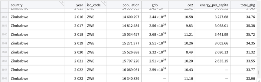
The foundation of any carbon tax analysis is comprehensive emissions data. For this study, I needed a dataset that covers multiple countries over a long time period, with information on both emissions and the economic factors that might influence them. The most essential variables for this empirical research project are CO2 emissions, population, GDP, and energy consumption patterns. As such, a dataset from Our World in Data’s CO2 and Greenhouse Gas Emissions database was retrieved to process this information.
The original dataset surprised me by extending all the way back to 1750, providing a very interesting perspective on carbon emissions patterns. It had many missing values for earlier periods, though, and required some cleaning. For the purposes of analyzing carbon tax effectiveness, I filtered the data to focus on 2001 onward. This timeframe captures the modern era of climate policy when carbon taxes actually started being implemented seriously. Earlier data, while historically fascinating, wouldn’t be relevant for studying carbon tax impacts since these policies have only been implemented fairly recently.
Import the comprehensive carbon emissions dataset, then filter for 1989-onward and choose essential variables essential for carbon tax impact analysis.
In[]:=
processedCarbonEmissionsRobust=Module[{data,tabularData,step1,step2},data=CloudGet[CloudObject[
https://www.wolframcloud.com/obj/7b374da8-7a42-408b-ab95-9112190c5df8
]];tabularData=ToTabular[data,"Rows",<|"HeaderRows"->1|>];step1=Select[tabularData,#year>=2001&];step2=step1[[All,{"country","year","iso_code","population","gdp","co2","energy_per_capita","total_ghg"}]];step2]Out[]=
Tax Data
Tax Data
Carbon tax policies are more complex than a simple yes/no variable. Different countries tax different fossil fuels at different rates, and these rates change over time. To capture this complexity, I needed detailed data on fuel-specific tax rates for coal, natural gas, and oil across all countries and years. As such, a dataset from a carbon pricing database developed at the University of Cambridge was retrieved to process this information. This dataset was originally developed within the Energy Policy Research Group at the University of Cambridge and represents the most comprehensive attempt at providing consistent cross-jurisdictional information on carbon pricing mechanisms introduced worldwide since 1990, including their sectoral and fuel coverage as well as associated price signals.
The raw tax data comes in a long format where each row represents a specific fuel type in a specific country-year. To make this usable for analysis, I restructured it into a wide format where each country-year has separate columns for coal, natural gas, and oil tax rates. I also created an average tax rate variable that captures the overall policy intensity across all fuel types. The tax column is a binary indicator that will be 0 if there are no taxes for a country-year and 1 if there is at least one tax.
Import and restructure carbon tax data from long to wide format, then create a column for average tax.
In[]:=
processedCarbonTaxesCountry=Module[{allData,removingDuplicates,pivotTo,rename,fill,mean,string,step1,step2,step3,step4,step5,normalised,cols,cleanList,cleanTabular},allData=Normal[ToTabular[CloudGet[CloudObject[
https://www.wolframcloud.com/obj/d406f541-f527-4555-8e02-5a40bb8cdc9
6
]],"Rows",<|"HeaderRows"->1|>]];removingDuplicates=Select[DeleteDuplicates[RenameColumns[ToTabular[allData],{"jurisdiction"->"country"}]],(!MissingQ[#Product])&];pivotTo=PivotToColumns[removingDuplicates,"Product"->"tax_rate_excl_ex_clcu"];rename=RenameColumns[pivotTo,{ExtendedKey["Coal"]->"coal",ExtendedKey["Natural gas"]->"naturalgas",ExtendedKey["Oil"]->"oil"}];fill=TransformColumns[rename,{"coal"->(If[MissingQ[#coal],0,#coal]&),"naturalgas"->(If[MissingQ[#naturalgas],0,#naturalgas]&),"oil"->(If[MissingQ[#oil],0,#oil]&)}];mean=TransformColumns[fill,"averagetax"->(Mean[{#coal,#naturalgas,#oil}]&)];normalised=Normal[mean];cols=Keys@First[normalised];cleanList=DeleteDuplicatesBy[SortBy[normalised,({-#["tax"],#["country"],#["year"],#["Product"],#["tax_rate_excl_ex_clcu"],#["tax_curr_code"]})&],({#["country"],#["year"]})&];cleanTabular=SortBy[Tabular[cleanList,cols],{"country","year","tax"}];cleanTabular]Out[]=
Tabular


Exchange Rate Data
Exchange Rate Data
To make meaningful comparisons of carbon tax rates across countries, it’s imperative to convert all tax values to a common currency. Carbon taxes are typically reported in local currencies - euros for European countries, dollars for the US, yen for Japan, etc. Without currency conversion, I can’t tell whether a 50 euro carbon tax is higher or lower than a 200 yuan carbon tax. The exchange rate data allows me to convert all carbon tax rates to a common baseline (US Dollars). As such, a dataset from the World Bank’s official exchange rate database was retrieved to process this information. This dataset provides the official exchange rate (LCU per US$, period average) which represents the exchange rate determined by national authorities or the rate determined in the legally sanctioned exchange market.
Import and process exchange rate data for currency conversions. Pivot from wide to long format for country-year observations and use string matching to extract numerical values.
In[]:=
exchangeRates=Module[{getData,step1,step2,step3,step4,step5,step6,step7,step8,step9},getData=CloudGet[CloudObject[
https://www.wolframcloud.com/obj/75abc1cd-6377-4f74-86d8-6a5fef06ed00
]];step1=ToTabular[getData,"Rows",<|"HeaderRows"->1|>];step2=Normal[step1];step3=Keys[First[step2]];step4=Select[Table[Which[StringMatchQ[ToString[variable],RegularExpression[".*\\d.*"]],ToString[variable],True,"ToBeRemoved"],{variable,step3}],#=!="ToBeRemoved"&];step5=PivotFromColumns[step1,step4->{"year","exchangerate"}];step6=step5[[All,{"Country Name","year","exchangerate"}]];step7=ToTabular[step6];step8=TransformColumns[step7,{"year"->(ToExpression[StringTake[#year,{5,8}]]&)}];step9=RenameColumns[step8,{"Country Name"->"country"}];step9] Out[]=
Tabular
Deforestation Data
Deforestation Data
Forests act as carbon sinks, absorbing CO2 from the atmosphere. When countries lose forest cover, they’re not only releasing stored carbon but also reducing their natural capacity to absorb future emissions. This makes tree cover loss an important variable to control for when analyzing carbon emissions patterns. I filtered the data to only include values where the canopy cover threshold was 30% or more. This is a standard cut-off used by Global Forest Watch and other environmental monitoring efforts to define true forested regions. As such, a dataset from Global Forest Watch was retrieved to process this information. The resulting dataset shows annual tree cover loss in hectares for each country-year.
Import and process tree cover loss data with 30% canopy threshold and pivot from wide to long format.
In[]:=
tcLossPerCountry=Module[{getData,step1,step2,step3,step4,step5,step6,step7},getData=CloudGet[CloudObject[
https://www.wolframcloud.com/obj/0722dee7-06e8-492f-ae88-5b0dd92a7655
]];step1=ToTabular[getData,"Rows",<|"HeaderRows"->1|>];step2=Select[step1,(#threshold===30)&];step3=Keys[First[Normal[step2]]];step4=Select[Table[Which[StringMatchQ[variable,RegularExpression[".*loss_ha_.*"]],variable,True,"ToBeRemoved"],{variable,step3}],#=!="ToBeRemoved"&];step5=PivotFromColumns[step2,step4->{"year","tcLossha"}];step6=TransformColumns[step5,{"year"->(ToExpression[StringTake[#year,{12,15}]]&)}];step7=step6[[All,{"country","year","tcLossha"}]];step7]Out[]=
Tabular
GDP Deflator Data
GDP Deflator Data
When comparing economic data across different years, inflation makes raw numbers misleading. A GDP of $1 trillion in 1990 represents much more real economic activity than $1 trillion in 2020 due to inflation. To make meaningful comparisons over time, I need to convert all monetary values to a common baseline using GDP deflators. As such, a dataset from the World Bank’s GDP deflator database was retrieved to process this information. GDP deflators are particularly important for this analysis because I’m looking at carbon tax rates over long time periods. A $20 carbon tax in 2005 had more of an effect than a $20 tax today. By using deflators, I can convert all tax rates and economic variables to constant dollars, making the analysis much more accurate.
The following dataset provides annual GDP deflator values for each country-year, allowing me to adjust for country-specific inflation patterns. Different countries experience different inflation rates, so using a single global deflator would introduce errors.
Import and process GDP deflator data for inflation adjustment, pivot from wide to long format.
In[]:=
gdpDeflator=Module[{getData,step1,step2,step3,step4,step5,step6,step7,step8,step9},getData=CloudGet[CloudObject[
https://www.wolframcloud.com/obj/fc74540b-2e3e-4786-8094-be3b5ebd4be5
]];step1=ToTabular[getData,"Rows",<|"HeaderRows"->1|>];step2=Normal[step1];step3=Keys[First[step2]];step4=Select[Table[Which[StringMatchQ[variable,RegularExpression[".*\\d.*"]],variable,True,"ToBeRemoved"],{variable,step3}],#=!="ToBeRemoved"&];step5=PivotFromColumns[step1,step4->{"year","gdpDeflator"}];step6=step5[[All,{"Country Name","year","gdpDeflator"}]];step7=ToTabular[step6];step8=TransformColumns[step7,{"year"->(ToExpression[StringTake[#year,{4,7}]]&)}];step9=RenameColumns[step8,{"Country Name"->"country"}];step9]Out[]=
Tabular
Meat Production Data
Meat Production Data
Livestock agriculture is a significant but often overlooked source of greenhouse gas emissions. Cattle, sheep, and grazers produce methane through digestion, while meat production more generally contributes to CO2 emissions through feed production, land use changes, and processing. Since agricultural emissions aren’t typically covered by carbon tax policies, I need to control for meat production to avoid attributing emission changes to carbon taxes when they might actually be driven by changes in agricultural activity. As such, a dataset from Our World in Data’s Agricultural Production database was retrieved to process this information. The following dataset tracks total meat production in tonnes for each country-year.
Import and process meat production data.
In[]:=
meatProduction=Module[{data,step1,step2},data=CloudGet[CloudObject[
https://www.wolframcloud.com/obj/8730edf1-19b2-4500-afc2-8cef6218fdc9
]];step1=ToTabular[data,"Rows",<|"HeaderRows"->1|>];step2=RenameColumns[step1,{"Entity"->"country","Code"->"iso_code","Year"->"year","Meat, total | 00001765 || Production | 005510 || tonnes"->"meatproduction"}];step2]Out[]=
Tabular
Merging & Cleaning Up Datasets
Merging & Cleaning Up Datasets
Merged Data
Merged Data
Once I had all of my data sources in one notebook, it was time to merge them into a unified dataset to use in my models. Only data from 2001 onward was retained, and I excluded entries with missing information, such as Djibouti. To enable fair cross-country comparisons, I used exchange rate data to convert tax values into USD. I also used the GDP deflator values to adjust for inflation, allowing both GDP and tax rates to be expressed in real dollars. At this stage, I decided which variables were truly relevant and removed any that were redundant. After transforming and renaming key columns, the resulting dataset includes: population, CO₂ emissions, energy consumption per capita, carbon tax policy intensity (in real USD), tree cover loss (filtered at 30% canopy), inflation-adjusted GDP, and meat production, all organized by country and year.
Merge all datasets using country and year and then adjust GDP and average tax.
I had to standardize units across variables to ensure consistency and interpretability. I converted energy per capita from megawatts per person to kilowatts, transformed tree cover loss from hectares to square meters, and scaled CO2 emissions out of millions to make the coefficients more readable in the regression output. I ended up with two nearly identical final models that differed only in how emissions were measured. In the second version (modelDataLogCO2), I replaced CO2 emissions with the natural log of CO2 emissions to improve the statistical properties for future regression models.
Remove all rows with missing values and adjust units for the other variables.
Replace the CO2 column with its natural logarithm.
Variables for the Econometric Models
Variables for the Econometric Models
◼
The country variable consists of string values and these represent the names of the countries from which the carbon emissions were made
◼
The year variable consists of integer values and shows the year of data collection
◼
The tax variable consists of real values (either 1 or 0) which are binary indications of whether or not there is a tax (1 for tax, 0 for no tax)
◼
The population variable consists of integer values representing the total population count for the country-year
◼
The CO2 variable consists of real values representing CO2 emissions in tons (or the natural logarithm of CO2 for modelDataLogCO2)
◼
The energy variable consists of real values representing energy consumption measured in kilowatt-hours per person.
◼
The tcLoss variable consists of real values representing tree cover loss in square meters
◼
The averagetax variable consists of real values representing the adjusted average tax in USD/ton of CO2 emissions
◼
The gdpreal variable consists of real values representing the inflation-adjusted GDP in USD
◼
The meatproduction variable consists of real values representing meat production in tons
Econometrics
Econometrics
Visualising time series before and after taxation
Visualising time series before and after taxation
For a very simple model of how carbon taxes correlate with emissions, I created a function which plots carbon emissions against time, in years, for a given country. Blue dots represent emissions before any tax is implemented, and orange dots represent emissions after its implementation.
Using the United Kingdom as an example, we can see that after a tax is implemented CO2 emissions continue to drop significantly in a generally downward trend.
This pattern isn’t unique to the UK. Let’s examine a few other examples:
Japan shows a similar pattern; emissions were relatively stable before carbon tax implementation, then show a clear downward trajectory afterward.
Chile presents an interesting variation on this theme. While emissions don’t drop as dramatically as in the UK or Japan, there’s a slight change in trajectory-what was previously a steep upward trend seems to level off after tax implementation. This suggests that carbon taxes can be effective even when they don’t immediately reverse emission trends, but rather slow or halt their growth.
Though the specific effects vary by country, these simple visualizations suggest that carbon taxation coincides with meaningful changes in emission patterns. However, they don’t control for other factors that might influence emissions trends. The regression models that follow will provide a more rigorous analysis that accounts for economic, environmental, and policy variables that could also explain these emission patterns.
Model 2 - CO2 Emissions & Average Tax
Model 2 - CO2 Emissions & Average Tax
Specify the model
Specify the model
Build a model using average tax rates instead of binary tax presence.
This model now gets more interesting; now we’re looking at actual tax rate levels instead of just presence/absence of tax. This makes more sense because carbon taxes can vary a lot—some countries have tiny rates that probably don’t change behavior much, while others have substantial taxes that might actually influence emissions.
See results
See results
Get the parameter estimates.
The intercept (239,316,482) represents baseline emissions when the average tax rate is zero. Most importantly, the averagetax coefficient is -1,896,853, which is negative as we’d expect: higher tax rates are associated with lower emissions. Similarly to the previous model, the p-value (0.098762) shows statistical significance at the 10% level, but not at the 5% level.
Get the adjusted R^2.
The adjusted R-squared of 0.000685566 is still extremely low (explains less than 0.1% of emission variation), to a comparable extent as in the previous model, suggesting that using taxation data does not provide sufficient information to explain variations in CO2 emissions.
Get the analysis of variance.
The F-statistic of 2.72744 shows this model is still not statistically significant overall, but it is improved since model 1.
Get variance inflation factors.
No multicollinearity concerns.
Plot
Plot
To facilitate the visualisation of this relationship, I built a function that can plot the tax-emission relationship for any individual country. This lets us see how carbon tax changes within a specific country correlate with emission changes over time, rather than just comparing across different countries.
Generate a plot showing the predicted relationship for a specific country
Below, I plotted the relationship for the Switzerland. The downward slope shows that as Switzerland’s carbon tax rates increased over time, emissions tended to decrease. The actual data points are scattered around the fitted line, which is normal - there’s always some noise in real-world data, but the overall trend is clear.
Model 5 - Log CO2 Emissions, Average Tax, Population, Energy, Tree Cover Loss, GDP, Meat Production, Country, Year
Model 5 - Log CO2 Emissions, Average Tax, Population, Energy, Tree Cover Loss, GDP, Meat Production, Country, Year
Specify model
Specify model
The final model includes country and year fixed effects. This is a big methodological step because it controls for any country-specific factors that don’t change over time (geography, culture, political systems) and any year-specific factors that affect all countries (global economic conditions, technological changes, international agreements). Essentially, this model only uses within-country variation over time to estimate the tax effect.
See results
See results
Get the parameter estimates.
The fixed effects model shows some interesting changes. The averagetax coefficient is -0.0018664 and remains statistically significant (p = 0.0001986439), confirming that carbon taxes reduce emissions even when we control for all time-invariant country characteristics and global year effects, although to a smaller extent. Put simply, for every additional USD taxed per ton of CO2 emitted, the fixed effects model expects CO2 emissions to fall by roughly 0.2%. Energy consumption remains highly significant with a large positive coefficient. Interestingly, many of the country fixed effects are negative, suggesting that after controlling for economic and environmental factors, most countries emit less than the baseline. The long list of country coefficients represents each country’s unique characteristics that don’t change over time. The fixed effects approach addresses the biggest concern with carbon tax research - that countries implementing carbon taxes might be systematically different from those that don’t. By using only within-country variation, we’re essentially asking: when a country increases its carbon tax rate, do its emissions go down? The answer appears to be yes.
Get the adjusted R^2.
The adjusted R-squared jumps to 0.999922, meaning this model explains over 99.99% of emission variation. This makes sense because country and year fixed effects capture most systematic variation in the data.
Get the analysis of variance.
Almost all variables remain highly significant (p-values essentially 0.0), including carbon tax, energy, population, GDP, and tree cover loss. Only meat production remains non-significant. Importantly, the year effects are also significant (p = 0.0000516778), confirming that there are global trends affecting all countries simultaneously.
Get variance inflation factors.
The VIF values are reasonable across all variables, but get a bit wonky with some reaching the hundreds. This is expected in fixed effects models with many dummy variables. The high VIF values are primarily due to the large number of country and year dummy variables, which naturally correlate with each other.
Create a visualization function.
This function allows us to examine the carbon tax effect for any specific country in any given year. I’m using Germany in 2018 as an example, but the function works for any country-year combination in our dataset. The plot shows the predicted relationship between carbon tax rates and log emissions for that specific country and year, holding all other variables (population, energy, GDP, etc.) at their mean values while fixing the country and year effects. The downward slope represents the estimated effect of carbon tax changes within that country during that time period, controlling for all the country-specific and year-specific factors that might confound a simple comparison across different countries or time periods.
Analyses of CO2 per capita
Analyses of CO2 per capita
Since countries vary dramatically in size, looking at total emissions can be misleading. A large country might have high total emissions simply because it has more people, not because it’s particularly carbon-intensive. To get a clearer picture of carbon efficiency, I analyzed CO2 emissions per capita - basically, how much each person in a country contributes to emissions on average.
1. Carbon Tax Impact
1. Carbon Tax Impact
Plot to visualize carbon tax impact on per-capita emissions for any country.
This plot shows the relationship between carbon tax rates and per-capita emissions across all countries that have implemented carbon taxes. The downward trend suggests that countries with higher carbon tax rates tend to have lower per-capita emissions, which supports the effectiveness argument. While there’s considerable scatter in the data points (reflecting the many other factors that influence per-capita emissions), the overall trend is clear.
2. Plot Variable v.s. CO2
2. Plot Variable v.s. CO2
I created a function that creates a regression model using energy per capita, tree cover loss, meat production, and average tax rate to predict CO2 per capita emissions. You can select which variable to examine while the function holds the other three variables constant at specified values.
A visualization function to examine relationships between a variable and CO2 per capita.
To use the function, you need to provide values for the three variables you’re not examining. I used the mean values for each, which represents average conditions across all countries.
Find the mean of energy, tree cover loss, meat production, and average tax.
Call plotVariableVsCO2 for energy.
The results show a strong positive relationship between energy consumption and per-capita emissions. The steep upward slope in the plot demonstrates that countries with higher energy consumption per capita tend to have significantly higher CO2 emissions per capita. The adjusted R-squared of 0.141198 indicates this model explains about 14% of the variation in per-capita emissions across countries. All variables in the regression are statistically significant, with energy consumption showing the strongest coefficient and highest significance. Interestingly, the positive coefficient on average tax seems counterintuitive. However, there may be some trade-offs to taxation when looking at per capita values of CO2. Which begs a question for future analysis, is there an optimal level of taxation for CO2 emissions?
3. Plot Variable v.s. CO2 per Country
3. Plot Variable v.s. CO2 per Country
I next created a function that does the exact same thing within a chosen country. By focusing on single countries, we can see how changes in energy use, deforestation, agricultural production, or tax policy correlate with emission changes over time within that specific context.
Build a country-specific visualization function to examine relationships within individual countries
To use this function, you need to provide values for the three variables you’re not examining. I used the mean values for each, but this time just the mean in the given country. But this flexibility is particularly powerful for country-specific analysis - if you’re studying a particular country with known characteristics (certain levels of meat production, energy usage, deforestation), you can input those exact values and see how different variables affect emissions within that country’s specific context.
Find the mean of energy, tree cover loss, meat production, and average tax in the chosen country (Switzerland).
Call plotVariableVsCO2Country for Switzerland and averagetax.
This plot indicates an effect of taxation that one would find more intuitive, at least when looking at the case of Switzerland. An additional USD taxed per ton of CO2 emitted, the model expects CO2 emissions per capita in Switzerland to fall by roughly 0.015 tons.
4. Plot Variable v.s. Log CO2
4. Plot Variable v.s. Log CO2
Similarly, I created a function that does the same thing but with log-transformed CO2 emissions because the log transformation helps address the skewed nature of emissions data and can reveal relationships that might be obscured in the raw data.
Build a comprehensive visualization function using log-transformed emissions
Call plotVariableVsLogCO2 for tcLoss.
This plot suggests that additional area of tree cover lost will increase CO2 emissions.
5. Plot Variable v.s. Log CO2 country
5. Plot Variable v.s. Log CO2 country
Finally, I created a function that does the same thing but combines country-specific analysis with log transformation because this approach is particularly useful when examining individual countries with very different baseline emission levels, as the log scale makes proportional changes more comparable
Build a country-specific visualization function using log-transformed emissions.
Find the mean of energy, tree cover loss, meat production, and average tax in the chosen country (Argentina).
Call plotVariableVsCO2Country for Argentina and meatproduction,
This plot shows that, in Argentina, additional meat production would not impact CO2 emissions significantly.
Conclusion
Conclusion
It can be argued that carbon taxation can be an effective tool for reducing CO2 emissions, though the magnitude and consistency of this effect varies significantly across different countries and analytical approaches. The regression models demonstrate that carbon taxes are associated with lower emissions even after controlling for economic factors like GDP and population, environmental variables like deforestation, and agricultural factors like meat production. This relationship remained statistically significant across multiple model specifications, from simple binary tax indicators to comprehensive fixed effects models that control for country-specific and time-specific factors. However, the effectiveness of carbon taxation is not uniform across all contexts. The time series visualizations revealed that while some countries like the United Kingdom and Japan experienced clear emission reductions following carbon tax implementation, others like Chile showed more modest effects where taxes appeared to slow emission growth rather than reverse it entirely. The per-capita analysis further demonstrated that carbon taxes correlate with lower emission intensity, suggesting they promote efficiency improvements rather than just absolute reductions. The fixed effects models, which provide the strongest causal evidence, showed that the carbon tax effect persists even when accounting for all time-invariant country characteristics and global trends. The analysis revealed, across various models, that carbon tax effectiveness depends heavily on the broader policy and economic context. The comprehensive models including energy consumption, economic development, and environmental factors confirmed that while carbon taxes contribute to emission reductions, they work alongside other important drivers of emission patterns. This emphasizes the need for integrated climate policies to reduce CO2 emissions rather than relying on taxation alone.
References
References
◼
Hannah Ritchie, Pablo Rosado, and Max Roser (2023) - “CO₂ and Greenhouse Gas Emissions” Published online at OurWorldinData.org. Retrieved June 29, 2025, from https://ourworldindata.org/co2-and-greenhouse-gas-emissions [Online Resource]
◼
Dolphin, G., Xiahou, Q. World carbon pricing database: sources and methods. Sci Data 9, 573 (2022). Retrieved July 1, 2025, from https://github.com/g-dolphin/WorldCarbonPricingDatabase
◼
World Bank. (2024). Official exchange rate (LCU per US$, period average) [Dataset]. World Bank Open Data. Retrieved July 5, 2025, from https://data.worldbank.org/indicator/PA.NUS.FCRF
◼
Global Forest Watch. (2024). Global Forest Change Data. World Resources Institute. Retrieved July 3, 2025, from https://www.globalforestwatch.org/dashboards/global/
◼
World Bank. (2024). GDP deflator (base year varies by country) [Dataset]. World Bank Open Data. Retrieved July 5, 2025, from https://data.worldbank.org/indicator/NY.GDP.DEFL.ZS
◼
“Data Page: Total meat production”, part of the following publication: Hannah Ritchie, Pablo Rosado, and Max Roser (2023) - “Agricultural Production”. Data adapted from Food and Agriculture Organization of the United Nations. Retrieved July 5, 2025, from https://archive.ourworldindata.org/20250624-125417/grapher/global-meat-production.html [online resource] (archived on June 24, 2025).
CITE THIS NOTEBOOK
CITE THIS NOTEBOOK
Model the impact of carbon tax policies on carbon emissions
by Amrita Kumar
Wolfram Community, STAFF PICKS, July 10, 2025
https://community.wolfram.com/groups/-/m/t/3502250
by Amrita Kumar
Wolfram Community, STAFF PICKS, July 10, 2025
https://community.wolfram.com/groups/-/m/t/3502250