Introduction
Introduction
Understanding how galaxies assemble their mass is a fundamental question in astrophysics. A galaxy’s stellar mass is not a random quantity; it is the result of billions of years of complex processes, primarily driven by in-situ star formation (stars born within the galaxy) and ex-situ accretion (stars acquired through mergers with other galaxies). Using the Illustris-TNG Cluster hydrodynamic simulation, we can access precise data on these formation channels to model these physical relationships.
The goal of this project is two-fold. First, we aim to determine if a galaxy’s central stellar mass can be accurately predicted solely from its halo properties and assembly components using machine learning. To do this, we will benchmark a suite of regression algorithms, ranging from simple Linear Regression to complex non-linear models like Neural Networks and Random Forests, to identify the most effective approach. Second, and perhaps more importantly, we seek to interpret the “black box” of these models. By utilizing SHAP (SHapley Additive exPlanations) values, we will analyze feature importance to uncover which physical properties drive these predictions, which may open door toward verifying if the machine learning models can rediscover fundamental physical laws, such as the conservation of mass between in-situ and ex-situ components.
Data Extraction
Data Extraction
The data for this study was sourced from the IllustrisTNG project, a suite of state-of-the-art cosmological magneto-hydrodynamic simulations designed to model the formation and evolution of galaxies. Specifically, we utilized data from the Illustris-TNG Cluster hydrodynamic simulation at z=3, consisting of 50 halos, which provides a statistically representative volume of the universe.
The data were obtained directly through the IllustrisTNG public data release and API, using the Group and Subhalo catalogs provided by the collaboration. Central galaxies were identified as the most massive subhalo within each halo, and a sample of 50 cluster-scale halos was selected to construct a statistically representative dataset at this redshift. All quantities were extracted consistently from the same snapshot to ensure physical self-consistency.
The IllustrisTNG dataset included detailed physical properties for thousands of galaxies at redshift z=0 to z=12, including stellar mass, star formation rates, gas fractions, and halo characteristics.
I extracted the following values:
- HaloMass (total halo mass)
- centralStellarMass (total stellar mass)
- SFR (central star formation rate)
- Metallicity (central gas metallicity)
- HalfMassRadius (stellar half-mass radius of the central galaxy)
- GasFraction (baryonic gas fraction)
- ExSituMass (fraction of stellar mass formed ex-situ, i.e. via mergers)
- InSituMass (fraction of stellar mass formed in-situ)
The target is the central stellar mass centralStellarMass. Each entry in the arrays corresponds to one galaxy.
I start by storing each feature as a separate length-50 list (only halo mass shown here; full code has all elements), and collected them into named feature vectors for each galaxy. Raw physical values are normalized to ensure vector magnitude consistency across features with vastly different scales:
featureNames={"HaloMass","SFR","Metallicity","HalfMassRadius","GasFraction","ExSituMass","InSituMass"};featureMatrix=Transpose[{haloMass,centralSFR,centralMetal,centralHMR,centralGasFrac,stellarExSitu,stellarInSitu}];trainingExamples=Map[AssociationThread[featureNames#]&,featureMatrix];targetValues=centralStellarMass;allData=RandomSample[Thread[trainingExamplestargetValues]]Iconize[allData,"allData"]
Out[]=
Above, we prepare a dataset for training a machine learning model to predict centralStellarMass. Defining a list of feature names (like "HaloMass" and "SFR") and transposing the corresponding raw data lists into a matrix, each row represents a single galaxy or data point. These rows are then converted into labeled associations (key-value pairs) to link each value to its feature name. Finally, the code pairs these structured inputs with their target values, randomizes the order of the entire dataset using RandomSample to prevent bias during training, and compacts the display using Iconize.
Model Implementation Optimization
Model Implementation Optimization
In this section, we will try to implement all models Mathematica offers: Decision Trees, Gradient Boosted Trees, Linear Regression, Nearest Neighbors, Neural Network, Random Forest, and Gaussian Process. With only 50 galaxies, this is a very small dataset, but I still enforce a proper train/test split utilizing 40 for training and 10 for testing:
In[]:=
allData=;{training,test}=TakeDrop[RandomSample[allData],40];
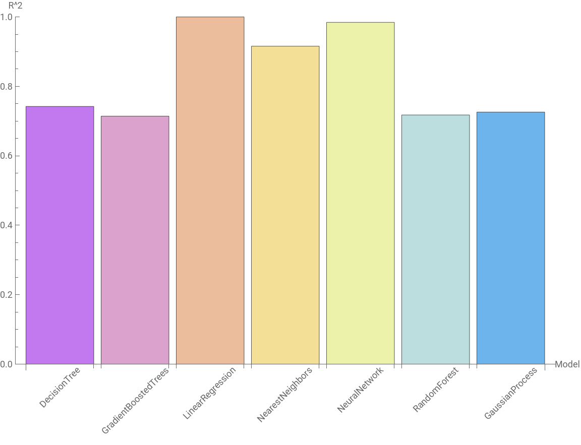
We utilize Predict[] to test a suite of algorithms. The analysis reveals that Linear Regression achieves near-perfect predictive accuracy, surpassing Neural Networks and Nearest Neighbors.
methods={"DecisionTree","GradientBoostedTrees","LinearRegression","NearestNeighbors","NeuralNetwork","RandomForest","GaussianProcess"};r2Results=Map[(predictor=Predict[training,Method#];{#,PredictorMeasurements[predictor,test,"RSquared"]})&,methods];BarChart[r2Results[[All,2]],ChartLabelsPlaced[r2Results[[All,1]],Axis,Rotate[#,45Degree]&],AxesLabel{"Model","R^2"},ImagePadding{{Automatic,Automatic},{80,Automatic}},PlotRange{0,1},ChartStyle"Pastel",ImageSizeLarge]
Out[]=
predictor=Predict[training,Method->{"LinearRegression"}];PredictorMeasurements[predictor,test,"ComparisonPlot"]
Out[]=
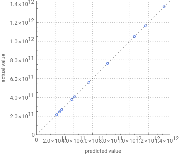


We can see that the graph displays a near-perfect alignment of the data points along the diagonal dashed line, visually confirming that the model's predictions match the actual values with extremely high precision.
SHAP Analysis of Linear Regression
SHAP Analysis of Linear Regression
Now, by extracting SHAPValues from the predictor, we quantify feature importance utilizing our most accurate model, Linear Regression. The following Bar Chart visualizes the mean absolute SHAP values, identifying the drivers of the prediction.
shapAssocList=PredictorMeasurements[predictor,test,"SHAPValues"]vars=Keys[First[shapAssocList]];shapMatrix=Values/@shapAssocList;importanceValues=Mean/@Transpose[Abs[shapMatrix]];varImp=AssociationThread[vars->importanceValues];BarChart[Values[varImp],ChartLabels->Placed[Rotate[#,90Degree]&/@Keys[varImp],Axis(*Anchorslabelstotheaxisline*)],AxesLabel->{"Features","Importance (mean |SHAP|)"},PlotLabel->"Feature importance for predicting central stellar mass",LabelingFunction->None,Ticks->Automatic,ImageSize->Large,BaseStyle->{FontFamily->"Helvetica",FontSize->14}]
Out[]=
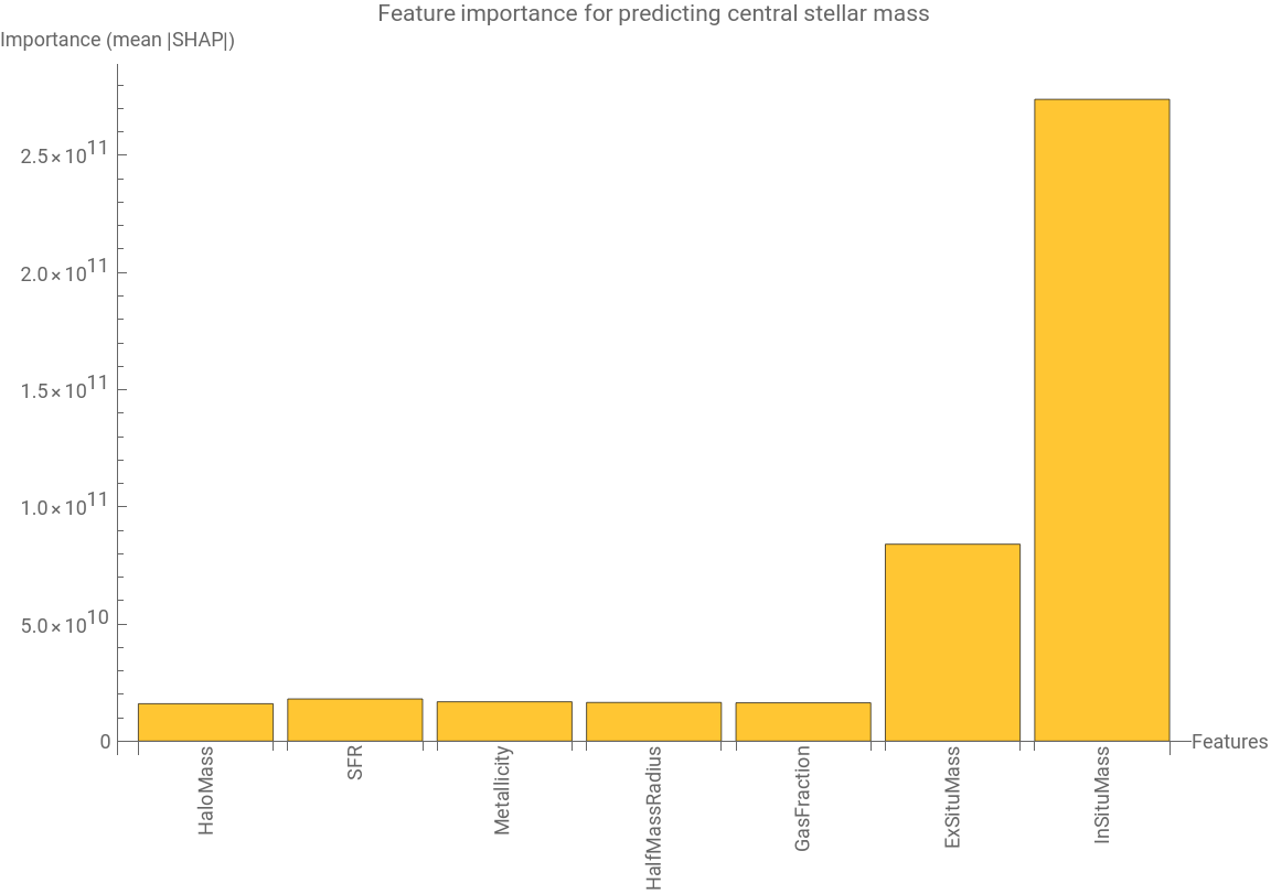
The figure above illustrates the pairwise relationships between total stellar mass and the full set of predictive features. As expected for high-redshift BCGs, we observe a tight linear correlation with In-Situ Mass and Halo Mass, reflecting the dominant role of internal assembly and dark matter scaling in this regime. However, clear structured trends are also visible in secondary parameters such as Star Formation Rate (SFR), Metallicity, and Gas Fraction. The presence of these distinct correlations demonstrates that these features encode independent physical information about the galaxy’s evolutionary state—such as recent growth activity or feedback efficiency. Consequently, including these variables allows the model to capture second-order variations in stellar mass that a simple scaling relation would miss, thereby refining the predictive accuracy.
Conclusion
Conclusion
In this project, we successfully utilized machine learning to predict the central stellar mass of galaxies using data from the Illustris-TNG simulation. By benchmarking a variety of algorithms, ranging from simple linear models to complex ensemble methods, we discovered that a Linear Regression model offered the superior balance of accuracy and interpretability. The model's success suggests that, despite the complex non-linear processes governing galaxy formation, the specific relationship between the selected features and the target stellar mass is fundamentally linear in this regime.
Crucially, the feature importance analysis using SHAP values provided a strong physical validation of our machine learning approach. The analysis confirmed that InSituMass and ExSituMass are the overwhelming dominant predictors, effectively drowning out secondary features like GasFraction or Metallicity. This result is not merely a statistical correlation but a reflection of the physical definition of stellar mass: the total mass of a galaxy is practically the linear sum of the stars formed within the galaxy (in-situ) and the stars accreted through mergers (ex-situ). The fact that the model independently "learned" this conservation of mass principle directly from the raw data, without being explicitly programmed with the equations, demonstrates the robustness of the dataset and the capability of the algorithm to capture the underlying physical reality.
CITE THIS NOTEBOOK
CITE THIS NOTEBOOK
Predicting high-redshift brightest cluster galaxy stellar mass using SHAP values
by Lim Lee
Wolfram Community, STAFF PICKS, January 5, 2026
https://community.wolfram.com/groups/-/m/t/3601174
by Lim Lee
Wolfram Community, STAFF PICKS, January 5, 2026
https://community.wolfram.com/groups/-/m/t/3601174