The whole study in one frame. Left: 50,000 simulated tournaments, with each team's title probability settling as the simulation count climbs. Right: the same forecast as a survival flow – the share of teams still alive thinning round by round, from 48 down to the champion.
A fully reproducible, self-contained study. We build an expected-goals (xG) model from StatsBomb open data – comparing frequentist machine learning with a Bayesian logistic model – then carry the uncertainty all the way to a Monte-Carlo forecast of the 48-team 2026 FIFA World Cup, with confidence intervals, scenario analysis, and a Bayesian vs frequentist comparison.
0. How to use this notebook
0. How to use this notebook
This notebook runs from a single folder. Put the three companion packages – wc_analysis.wl, tournament_data.wl and backtest.wl – in the same directory as this notebook, then Evaluation → Evaluate Notebook. Every figure and number after the setup is produced by a short, fully-argumented function call you can read, edit, and re-run.
The author's own inputs (team Elo ratings, the group draw, the 2018/2022 results, and de-vigged market odds – all factual) are embedded in the iconised cell below and written to a local data/ folder on the first run. The one dataset we may not redistribute is StatsBomb's shot-event data: under the StatsBomb Public Data User Agreement it cannot be shared, so the setup cell downloads it directly from StatsBomb (pinned to a fixed commit) and rebuilds the identical shot table locally – a one-time fetch of ~300 matches that takes a few minutes. A full run also does 50,000-tournament Monte-Carlo simulations twice and trains three classifiers; for a fast pass set $WCQuickMode = True below.
The author's own inputs (team Elo ratings, the group draw, the 2018/2022 results, and de-vigged market odds – all factual) are embedded in the iconised cell below and written to a local data/ folder on the first run. The one dataset we may not redistribute is StatsBomb's shot-event data: under the StatsBomb Public Data User Agreement it cannot be shared, so the setup cell downloads it directly from StatsBomb (pinned to a fixed commit) and rebuilds the identical shot table locally – a one-time fetch of ~300 matches that takes a few minutes. A full run also does 50,000-tournament Monte-Carlo simulations twice and trains three classifiers; for a fast pass set $WCQuickMode = True below.
wcEmbeddedData=
(*Self-containedsetup.Keepwc_analysis.wl,tournament_data.wlandbacktest.wlinthisnotebook'sfolder;everythingelseisbelow.*)dataDir=FileNameJoin[{NotebookDirectory[],"data"}];If[!DirectoryQ[dataDir],CreateDirectory[dataDir]];(*1.writeouttheembeddedfactualinputs(Elo,draw,results,marketodds)*)KeyValueMap[Export[FileNameJoin[{dataDir,#1}],#2,"Text"]&,Uncompress[First[wcEmbeddedData]]];(*2.pointtheengineatthisfolder,thenloadit*)$WCDataDirOverride=dataDir;Get[FileNameJoin[{NotebookDirectory[],"wc_analysis.wl"}]];Get[FileNameJoin[{NotebookDirectory[],"backtest.wl"}]];(*3.StatsBombshotdataisNOTredistributable(StatsBombPublicDataUserAgreement)–download+builditlocallyonfirstrun(afewminutes)*)ensureShotData[];"Ready • "<>ToString[Length[Names["WCAnalysis`*"]]]<>" functions; data in "<>dataDir
Ready • 52 functions (build)
The flag below controls run length. Leave it False to reproduce the published 50,000-run numbers; set it True for a fast (~1 minute) pass that caps every simulation at $WCQuickSims runs. (It lives in its own cell so it is set after the package is loaded.)
$WCQuickMode=False(*True→fastpass*)
False
The package exposes a small vocabulary of functions – simulateTournament, matchProbabilities, trainXGModels, bayesianLogisticXG, and a family of plot functions. Here is the full public API:
Multicolumn[Sort@Names["WCAnalysis`*"],3]
advMatchProbs | plotBayesVsFreq | plotTournamentFlow |
bayesianLogisticXG | plotCalibration | plotWinProbabilities |
bayesXGPredict | plotConfederations | plotXGMarginals |
betaBinomialCalibration | plotExpectedBracket | prepareXGData |
bootstrapCI | plotGroupHeatmap | proportionCI |
buildShotData | plotHostCities | scenarioTable |
calibrateToMarket | plotMarketComparison | simulateTournament |
ensureShotData | plotMatchProbabilities | teamProfile |
exitRoundTable | plotModelComparison | trainXGModels |
exportCalibratedRatings | plotNonTransitiveCycle | wilsonInterval |
loadShots | plotProgress | $WCBaseElo |
marketCalibrationTable | plotProximity | $WCDataDir |
marketProbs | plotScenarioComparison | $WCHostNations |
matchProbabilities | plotShotDensity | $WCProximity |
multiSeedWinCI | plotShotMap | $WCQuickMode |
nonTransitiveTriples | plotStyleSpace | $WCQuickSims |
plotAttackDefence | plotSurvivalHeatmap | |
plotBayesCalibration | plotTeamStrength | |
1. What is expected goals (xG)?
1. What is expected goals (xG)?
Expected goals (xG) assigns every shot a probability of becoming a goal given the circumstances in which it was taken: how far out, at what angle, with which body part, under how much defensive pressure. A central tap-in might be worth xG ≈ 0.7; a speculative 30-yard strike xG ≈ 0.03. Summing xG across a match gives the expected goal tally – comparing it with the actual score reveals who over- or under-performed relative to chance quality.
xG is now a modern standard for separating finishing from chance creation, and the same shot-probability idea transfers to hockey, basketball, and rugby. In this notebook xG does double duty: it is both the object of study (how well can we model it, and how certain are we?) and a sanity check on the team-strength ratings that drive the tournament simulation.
xG is now a modern standard for separating finishing from chance creation, and the same shot-probability idea transfers to hockey, basketball, and rugby. In this notebook xG does double duty: it is both the object of study (how well can we model it, and how certain are we?) and a sanity check on the team-strength ratings that drive the tournament simulation.
2. The 2026 FIFA World Cup
2. The 2026 FIFA World Cup
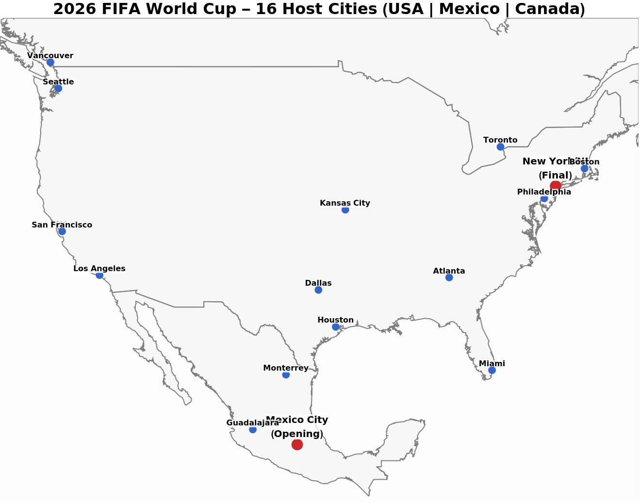
2026 is the first 48-team World Cup (up from 32), co-hosted by the USA, Canada, and Mexico across 16 cities, 11 June – 19 July 2026. The 48 teams are drawn into 12 groups of four; the top two of each group plus the eight best third-placed teams advance to a round of 32, then it is single-elimination to the final at MetLife Stadium, New York/NJ. That is 104 matches in all.
plotHostCities[]
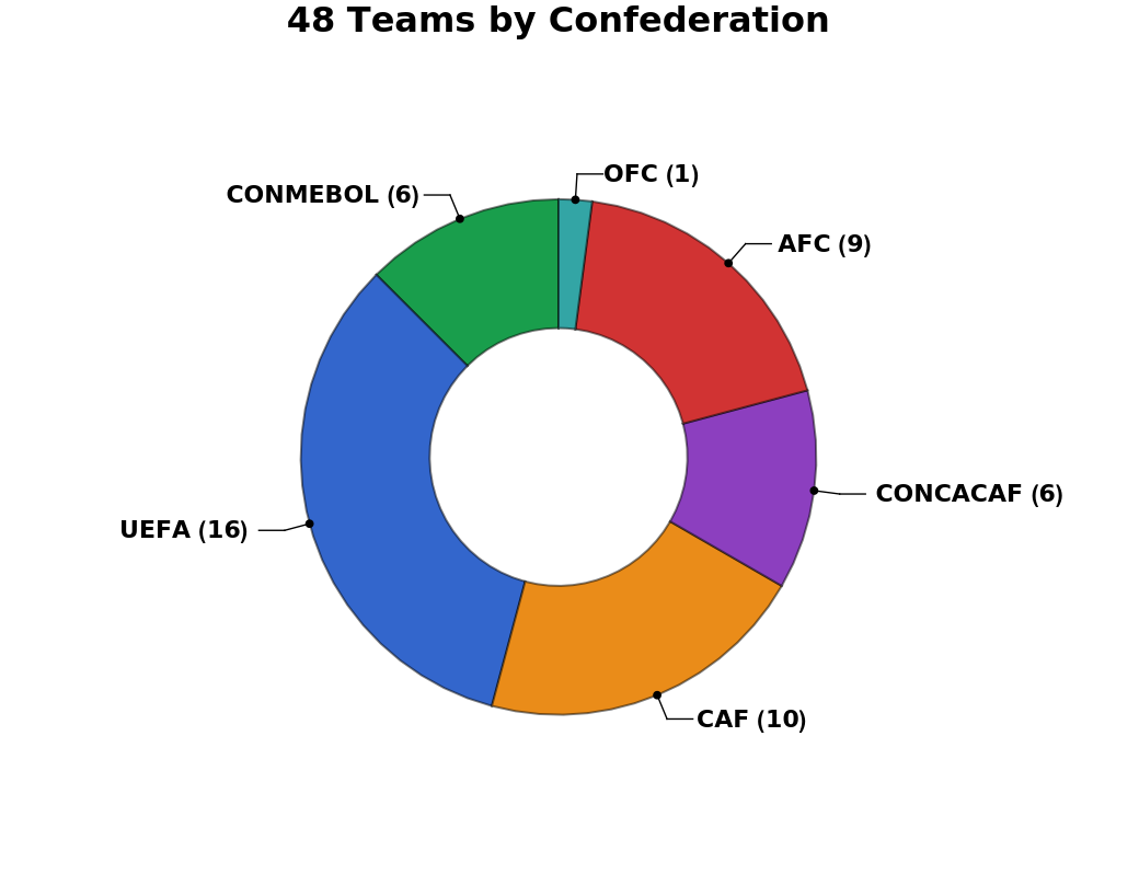
The 48 qualified teams span all six confederations. UEFA (Europe) and CAF (Africa) dominate the field by count; CONMEBOL (South America) is small but punches far above its weight in strength.
plotConfederations[]
3. Team strength: FIFA points and Elo
3. Team strength: FIFA points and Elo
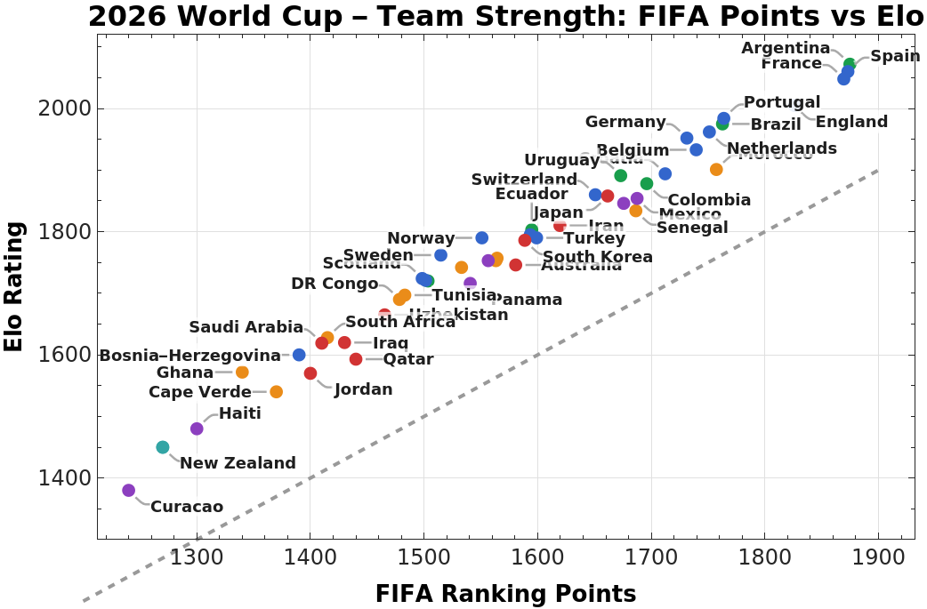
We summarise each team with two numbers: its FIFA ranking points (FIFA's own published rating) and its World-Football Elo rating (a result-based rating in the chess tradition). The two largely agree, which is reassuring, but they disagree at the margins – Elo, being purely result-driven, tends to reward teams on recent winning streaks. The simulation engine uses Elo, because the Elo expected-score formula maps cleanly onto win probabilities.
plotTeamStrength[]


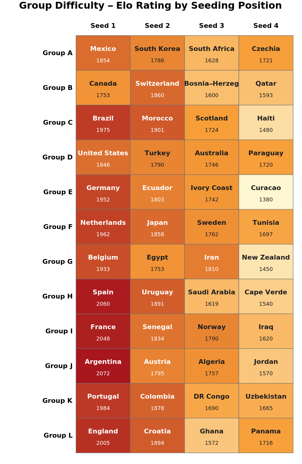
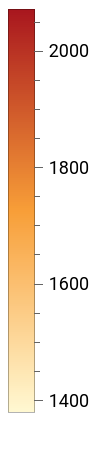
A draw is only as kind as its toughest opponents. The heatmap below shows every group's four teams ranked by Elo. Group H (Spain) and Group J (Argentina) are the classic 'groups of death' by top seed, while the gap between seeds 1 and 4 measures how lopsided each group is.
plotGroupHeatmap[]
4. StatsBomb open data and the shot table
4. StatsBomb open data and the shot table
StatsBomb publish event-level data – every pass, shot, and tackle with coordinates – for a large set of matches under their free Public Data User Agreement. From ~300 matches we extract every shot, with its location, body part, play pattern, the StatsBomb xG, and a freeze-frame count of defenders between shooter and goal. Penalties are removed (they are a fixed-probability special case that would distort the model). The shot table holds 7,381 usable shots at an 11.1% conversion rate. StatsBomb data is not redistributed here – the setup cell downloaded it directly from StatsBomb and rebuilt this table locally; we credit StatsBomb as required:
We summarise the danger as a heatmap rather than plotting individual shots: a smooth kernel regression of the model's predicted xG over pitch location. It recovers the familiar picture – danger concentrates in a tight cone around the six-yard box and falls off sharply with distance and angle. (Showing the smoothed field rather than the raw shots also keeps the figure an aggregate statistic, not a copy of StatsBomb's data.)
5. A frequentist xG model: three classifiers compared
5. A frequentist xG model: three classifiers compared
From each shot we build eleven features: distance, the angle subtended by the goal, number of defenders, the non-linear terms distance² and log(angle), a distance×angle geometry interaction, one-hot body-part indicators (right foot / left foot / head, rather than a fake numeric scale), and set-piece / counter-attack flags. We train three Wolfram Classify models on an 80/20 train/test split and score them on the held-out shots.
◼
Brier score (lower is better) – mean squared error of the probabilities.
◼
Log loss (lower is better) – penalises confident mistakes heavily.
◼
AUC (higher is better) – ranking ability: P(a random goal was rated above a random miss).
Crucially we do not report point estimates alone. The Brier score and AUC each come with a 95% bootstrap confidence interval (resampling the test set 400 times), so we can see whether the models are really distinguishable; log loss is shown alongside as a point estimate. They are barely distinguishable: the intervals overlap heavily, a useful reminder that 1,477 test shots is not a lot.
A model can have good discrimination (AUC) yet still be mis-calibrated – its probabilities systematically too high or too low. The calibration curve bins shots by predicted xG and plots the observed conversion in each bin against the 45° line. Gradient-boosted trees track the diagonal best; the random forest is noticeably over-confident in the mid-range.
6. A Bayesian xG model
6. A Bayesian xG model
The classifiers above give a single number per shot. A Bayesian model instead gives a posterior distribution, which propagates honestly into a credible interval on every xG. We fit a Bayesian logistic regression on an interpretable feature subset {distance, angle, defenders, is-header, is-set-piece} with a weakly-informative Gaussian prior, using IRLS to find the posterior mode (MAP) and a Laplace (Gaussian) approximation for the posterior covariance.
The fitted coefficients are physically sensible: distance lowers xG, a wider angle raises it, more defenders and headers lower it. The sign and magnitude of each effect now comes with quantified uncertainty.
The fitted coefficients are physically sensible: distance lowers xG, a wider angle raises it, more defenders and headers lower it. The sign and magnitude of each effect now comes with quantified uncertainty.
Because we have a full posterior, predicting the xG of a specific chance returns a mean and a 95% credible interval – not just a point. Compare a good chance (12 yards, central, open play) with a poor one (28 yards, tight angle).
The real payoff is the marginal-effect plot. The Bayesian model gives a smooth xG-vs-distance (and xG-vs-angle) curve with a shaded 95% credible band; overlaid is the gradient-boosted curve. The contrast is instructive: the Bayesian curve is smooth and admits its uncertainty, while the tree ensemble is flexible but steps and flattens where data thin out. Neither is 'right' – they encode different assumptions.
We can also recast calibration in Bayesian terms. For each predicted-xG bin, the observed conversion is k goals from n shots; a conjugate Beta(1+k, 1+n−k) posterior gives a 95% credible interval on the true conversion rate. Bins near the diagonal with intervals that straddle it are well-calibrated; the wide intervals at high xG simply reflect how few such chances exist.
7. From ratings to match outcomes
7. From ratings to match outcomes
To simulate a tournament we need a match model. We use the standard Elo expected-score curve to turn a rating gap into an expected score for team A, then spread an average of 2.5 goals per match across the two teams and draw each team's goals from an independent Poisson distribution.
From those two Poisson distributions we read off the exact win / draw / loss probabilities for any fixture (summing over score lines). A few headline group matches:
Two refinements make the match model more faithful, both available as options. First, the plain mapping λ = 2.5 E\_A treats the Elo expected score as a goal share, which is not self-consistent: the win/draw/loss it implies do not reproduce E\_A. The COHERENT mapping instead solves for the goal split so the Poisson expected result equals the Elo number exactly. Second, real football has more low-scoring draws than independent Poisson predicts – a Dixon-Coles correction (ρ) adds that low-score dependence. Compare the three for one fixture (note the coherent win probability drops toward the honest Elo value, and Dixon-Coles lifts the draw):
The model's assumptions are worth stating plainly (see also the limitations section):
◼
Goals are conditionally independent Poisson – no explicit modelling of game state, red cards, or score-dependent tactics.
◼
A fixed 2.5 goals/match scale (roughly the historical World-Cup average); we test sensitivity to this later.
◼
No home advantage by default – notable given three host nations; tested as a scenario.
◼
Elo ratings are treated as fixed and exact in the frequentist run – relaxed in the Bayesian run.
8. Monte-Carlo tournament – the frequentist forecast
8. Monte-Carlo tournament – the frequentist forecast
We now play the whole tournament – group stage, the best-third-placed bookkeeping, and the single-elimination bracket with extra time and penalties – tens of thousands of times, counting how often each team reaches each stage. With fixed Elo ratings this is a purely frequentist Monte-Carlo experiment: the only randomness is match variance.
A Monte-Carlo probability is itself an estimate, so we attach a 95% Wilson confidence interval to every bar: with N draws, a probability p has standard error ≈ Sqrt[p(1−p)/N]. At 50,000 runs the favourites are pinned to within about ±0.4 percentage points – tight enough to separate the top three from the chasing pack, but not enough to rank them confidently against each other.
The single 'win probability' number hides the structure of a deep run. The stacked view below shows, for the top contenders, the probability of reaching each successive stage – how steeply each team's curve falls from 'reach the knockouts' down to 'lift the trophy'.
The same object also answers group-level questions – for instance, each team's probability of escaping its group:
When does each team drop out?
When does each team drop out?
The win-probability bar chart only shows the favourites, but the simulation knows the fate of all 48 teams – including the ones that exit early. The survival heatmap shows every team's probability of reaching each round, from the group stage to the trophy. Read a row left to right to watch a team's chances fade: the colour drains out at the round where they most likely go home. Scotland, for example, is roughly a coin-flip to escape its group and almost never survives the round of 16.
The same survival, read as a flow. Every team enters at the group stage on the left; each ribbon thins round by round as its probability of advancing falls, so the field of 48 funnels down to a single champion on the right. The column totals are the expected number of survivors at each stage – 48 → 32 → 16 → 8 → 4 → 2 → 1 – so each knockout round roughly halves the bracket. The favourites' coloured ribbons run along the bottom and persist longest; the grey field above them drains away early.
The same information as a sortable, exact table – every team, its probability of reaching the round of 16 / quarter-final / semi-final, its title odds, its median finish (the round by which it is more likely than not eliminated), and the expected number of knockout rounds it survives (0 = out in the group stage, 6 = champion).
A subtlety worth spelling out. Argentina is the single most likely champion (≈ 21%), yet its likeliest single exit is its very first knockout game: it almost always reaches the round of 32 (only ≈ 0.5% exit in the group), and one-off knockout football always carries upset risk, so "lost in the round of 32" (≈ 26%) is a bigger single bucket than "won the whole thing" (≈ 21%) – winning requires surviving six straight knockout games. Both are true at once, which is why we report the median finish (Argentina, Spain and France all → quarter-final) rather than the misleading modal one. The expected-rounds-survived column is the most stable summary of all: France (3.6) actually edges Argentina (3.4), even though Argentina lifts the trophy more often.
The predicted bracket
The predicted bracket
Finally, the single most-likely picture: the chalk knockout bracket. Seeding each group by Elo and advancing the favourite at every step traces one deterministic path from the round of 32 to the final. It is only the most probable branch – the heatmap above is the honest probabilistic summary – but it is the cleanest way to see the whole tournament as a tree.
9. The Bayesian forecast: propagating rating uncertainty
9. The Bayesian forecast: propagating rating uncertainty
The frequentist run pretends the Elo ratings are exact. They are not – a rating is an estimate that drifts by tens of points from window to window. A Bayesian forecast treats each team's true strength as uncertain: θᵢ ~ Normal(Eloᵢ, σ), with σ ≈ 45 Elo points reflecting typical rating volatility. For every simulated tournament we first draw a fresh set of strengths from this prior, then play the matches. The result is a posterior-predictive distribution that carries both sources of uncertainty – match variance and parameter uncertainty – not just the first.
Comparing the two forecasts side by side shows the signature of parameter uncertainty: the Bayesian probabilities are flatter – favourites are pulled down and mid-tier teams pushed up – because in some draws the underdog is genuinely stronger than its point rating suggests. The gap between the blue and orange bars is, in effect, the cost of pretending we know each team's strength exactly.
Which forecast should you believe? If you trust the Elo ratings as gospel, the frequentist run is the conditional answer. If you accept that ratings are noisy – which they demonstrably are – the Bayesian run is the more honest unconditional forecast, and its wider, flatter distribution is a feature, not a bug.
10. Scenario analysis
10. Scenario analysis
A single forecast is fragile; a good one is stress-tested. We re-run the tournament under deliberate changes to the assumptions and watch which conclusions hold. All scenarios share a seed so differences are signal, not noise.
10a. Host advantage and goal environment
10a. Host advantage and goal environment
What if the three host nations enjoy a home boost (we add 60 Elo points, a typical home-field value)? What if 2026 is a high-scoring tournament (3.0 goals/match) rather than an average one (2.5)?
The takeaways are robust and intuitive: a host boost lifts the USA, Mexico, and Canada markedly while barely touching the favourites; a higher goal environment sharpens the gap between strong and weak teams (more goals = less variance = the better team wins more often), while a low-scoring tournament is the underdog's friend.
10b. How much does rating uncertainty matter?
10b. How much does rating uncertainty matter?
The Bayesian forecast hinges on one choice: σ, the assumed rating uncertainty. Sweeping it from 0 (= frequentist) upward shows how the favourite's win probability erodes as we admit more doubt about the ratings – a clean picture of the favourite-flattening effect, and a guide to how much it would move if you believe ratings are more or less reliable than 45 points.
11. Beyond Elo: non-transitivity, strengths & weaknesses, and home support
11. Beyond Elo: non-transitivity, strengths & weaknesses, and home support
Everything so far rests on a single Elo number per team. That buys simplicity but bakes in two questionable assumptions. First, Elo is strictly transitive: if A outrates B and B outrates C then A must be favoured over C – there is no room for the rock-paper-scissors matchups football fans know are real (1 beats 2 beats 3 but 3 beats 1). Second, one number cannot separate a team's attacking flair from its defensive solidity, nor capture that some teams are literally closer to home. The advanced model adds three transparent factors on top of Elo. Proximity is fully data-driven; the style and attack/defence pieces are honest, tunable parameterisations to stand in for the per-team event data we lack for all 48 nations.
1. Home support from real geography
1. Home support from real geography
Using the great-circle distance from each country to the nearest of the 16 host cities, we turn proximity into an Elo-point bonus, with a top-up for the three host nations. Mexico, the USA and Canada lead, then their CONCACAF neighbours and the South American sides; Asia and Oceania are effectively away from home.
2. Strengths and weaknesses: attack vs defence
2. Strengths and weaknesses: attack vs defence
Each team is split into an attack and a defence rating around its Elo by an "attacking lean": a high-lean side (Spain, Brazil, the Netherlands) scores and concedes more; a low-lean side (Morocco, Iran, Uruguay) is built to stifle. Two attack-minded teams produce a higher-tempo, higher-scoring game. Teams above the diagonal are attack-leaning, below it defence-leaning.
The full per-team profile – Elo, attack, defence, style angle, and home-support bonus:
3. Non-transitivity: a genuine rock-paper-scissors
3. Non-transitivity: a genuine rock-paper-scissors
Finally, each team sits at an angle on a "style circle", and a matchup term κ sin(θ\_i − θ\_j) tilts close games. Because the sine is antisymmetric – and we centre the matrix so no team gains a net advantage – it is purely cyclic: it cannot be collapsed into any ranking. Opposite styles counter each other; neighbours play alike.
The payoff is real intransitivity. Searching the top sides turns up genuine cycles where A is more likely to beat B, B to beat C, and C to beat A – something a single Elo ranking can never produce. Home support tilts some edges, so a host or near-host side can beat a team it would "rank" below.
Putting it together
Putting it together
Running the whole tournament under the advanced model and comparing with pure Elo shows the net effect: the hosts and their neighbours climb sharply on home support, while scoring profiles and style matchups reshuffle the chasing pack. Reassuringly, the three favourites remain the three favourites – the extra structure adds realism without overturning the headline. The honest summary is still the probabilistic one; this section shows the machinery you would feed with richer per-team data.
12. Mapping the betting market
12. Mapping the betting market
Every forecast so far is built from one number per team – Elo. That single number is blind to squad value, injuries, qualification form, the age of a defending-champion squad, and the odd generational striker. The betting market prices all of it in. We can fold those unseen factors in wholesale: treat the de-vigged market title odds as data and solve for the per-team effective ratings whose simulated title probabilities reproduce the market. The crucial part is that the simulation still plays the real draw and bracket – so this maps the market while keeping every path interaction. 'Given this group and this side of the bracket, who advances' remains a Monte-Carlo answer, not a flat copy of the market list.
The market odds – de-vigged Kalshi prediction-market prices cross-checked against sportsbook outrights (June 2026) – ship with the repository and expand to a probability over all 48 teams (the long tail of unlisted sides shares the residual mass by Elo strength):
Calibration is a damped fixed-point in log-odds space: simulate, compare each team's title chance with the market, nudge its rating toward the gap, repeat. A fixed random seed is used across iterations on purpose (common random numbers, so the objective is smooth); the curve below is therefore the in-sample training distance, which collapses from the raw-Elo starting point toward the Monte-Carlo noise floor within a dozen-odd iterations.
The fitted ratings differ from Elo by exactly the amount the market disagrees with a pure result-based rating – so the adjustment column is a direct readout of 'everything Elo misses'. The defending champions Argentina take the largest mark-down (Elo's top side, but the market doubts a repeat with an ageing squad); Belgium and Croatia are softened too; while Norway is marked up (a rating cannot see one generational striker) and the host nations hold their ground on home support.
Running the whole tournament with the calibrated ratings – on an independent random seed, so the agreement is a genuine out-of-sample check rather than the fit reproducing its own noise – recovers the market's title probabilities closely, while preserving every bracket interaction the market list throws away:
Two honest caveats. First, the calibration is fitted to title odds only: 48 ratings constrained by ~17 published championship prices (plus an Elo-imputed tail) is an under-determined inverse, so the fitted ratings are the simplest market-consistent adjustment, not a unique decomposition – read the per-team deltas as indicative. Second, every round-by-round figure elsewhere in this notebook (the progress bars, survival heatmap, flow diagram and exit table) deliberately uses the pure-Elo frequentist run, not these calibrated ratings, because the market prices we have constrain only the champion, not the earlier rounds.
With that said, the four forecasts are complementary, not rivals: the pure-Elo run says what results-based ratings alone imply; the Bayesian run adds honest rating uncertainty; the advanced model adds interpretable structure (home support, style, attack/defence); and this calibrated run imports the market's collective judgement. All four run on the same engine and the same draw, so the differences between them are exactly the assumptions you choose to believe.
With that said, the four forecasts are complementary, not rivals: the pure-Elo run says what results-based ratings alone imply; the Bayesian run adds honest rating uncertainty; the advanced model adds interpretable structure (home support, style, attack/defence); and this calibrated run imports the market's collective judgement. All four run on the same engine and the same draw, so the differences between them are exactly the assumptions you choose to believe.
The under-determination has a standard remedy: ridge-regularise the rating deltas toward base Elo with the Shrinkage option (calibrateToMarket[..., "Shrinkage" -> 0.05]), which tames the noisy long tail while leaving the well-determined favourites almost untouched; and reach-round market prices, if available, can be added to the objective via ExtraTargets. Finally, the fitted ratings are a reusable artefact, so we persist them – with provenance – to the repository:
13. Does the engine actually work? A backtest
13. Does the engine actually work? A backtest
A forecast you cannot check is just an opinion. The honest test is to run the same match model – the EloPoisson scoring and knockout logic used throughout – on past World Cups, scoring its predictions from each tournament's pre-tournament Elo against what actually happened. (The headline forecast is a 48-team bracket; the backtest reuses that match model in a small self-contained 32-team simulator matching the 2018/2022 format.) We backtest 2018 and 2022, each with pre-tournament ratings, the real draw, and every team's actual finishing round, embedded above and provided by the companion package backtest.wl loaded in the setup cell.
For each tournament we simulate from the pre-tournament ratings and score the predicted reach-round probabilities against reality with the Brier score (mean squared error of the probabilities) and log-loss, alongside a naive equal-chance baseline:
The engine beats the naive baseline by a clear Brier-skill margin, and the eventual winners sit near the top of its pre-tournament board – Argentina (2022) and France (2018) were both among the handful of favourites, not runaway picks, which is exactly how knockout football behaves. Pooling every team-by-round prediction gives a calibration curve: a point near the diagonal means that when the model said p, it happened about p of the time.
And the 2018 detail – predicted reach-round probabilities versus the actual finish. It shows the model's honest limitation too: it gave 2018 Germany (a very high pre-tournament Elo) strong odds, and Germany crashed out in the group stage. No rating-based model foresees that; the backtest is how we keep ourselves honest about it.
The 2022 detail tells the complementary story. The engine had Brazil and Argentina at the top of the board, and Argentina – a genuine favourite rather than a long shot – duly won, consistent with the model ranking it among the handful of favourites (the formal calibration evidence is the pooled curve and Brier skill above, not any single result). But the same table records the upsets no rating model can anticipate: Morocco, given modest reach-round odds, ran to the semi-finals, while several higher-rated sides exited early. The two tournaments together – a favourite delivering in 2022, a favourite collapsing in 2018 – are exactly why we score the engine over many simulations rather than trusting any single bracket.
14. Assumptions, limitations, and validity
14. Assumptions, limitations, and validity
This is a deliberately simple, transparent model. Honesty about what it does not do is part of the science.
◼
Independence of goals. Real matches have momentum, red cards, and score-dependent tactics; the headline run uses conditionally-independent Poisson goals. A Dixon-Coles low-score correction and a coherent Elogoals mapping are available as options (Section 7); they are kept off the headline for transparency.
◼
Fixed goal scale. 2.5 goals/match is a tournament-average constant, not team-specific attack/defence strengths. Section 10 shows the forecast is only mildly sensitive to it.
◼
Elo as the sole strength signal in the headline forecast. We do not directly use squad value, injuries, qualification form, or the xG ratings we built. Section 11 adds interpretable structure (proximity, attack/defence, non-transitive style), and Section 12 folds in everything at once by calibrating to the market – but the headline frequentist and Bayesian runs remain deliberately Elo-only so their assumptions are transparent.
◼
Bracket. Third-placed teams are routed to round-of-32 slots respecting FIFA's published per-group eligibility for each slot (a valid bipartite matching); the only remaining simplification is the deterministic tie-break among equally-valid matchings, which barely affects aggregate win probabilities.
◼
Calibration of σ. The Bayesian σ = 45 is a reasoned default from historical Elo volatility, not a fitted quantity; Section 10b shows its influence explicitly.
◼
Monte-Carlo error. All probabilities are estimates; the reported Wilson and bootstrap intervals quantify it, but the tails (a specific minnow winning) are the least precise.
Within those limits the model is well-behaved: the xG model is competitive with published work (AUC ≈ 0.79), the match probabilities are sensible, the tournament favourites match bookmaker and Opta-supercomputer consensus, and – crucially – the engine beats a naive baseline when back-tested on the 2018 and 2022 World Cups (Section 13).
15. Conclusions
15. Conclusions
Built entirely in the Wolfram Language from open data, this study shows a full pipeline: parse StatsBomb shots, model xG two different ways, and forecast a 48-team tournament with quantified uncertainty.
The headline forecast puts Argentina, Spain, and France clear of the field, with England the best of the rest – but the more important message is in the error bars. The three favourites are statistically inseparable, and the Bayesian forecast, by admitting that the ratings themselves are uncertain, flattens the field in a way that a naive point forecast hides. Calibrating the same engine to the betting market (Section 12) tells the complementary story: the market doubts a back-to-back Argentina, rates Norway well above its Elo, and rewards the hosts – precisely the squad-level knowledge a single rating cannot hold. Comparing frequentist, Bayesian, and market-calibrated answers – at both the shot level and the tournament level – is the most honest way to report a prediction: not a single number, but a distribution with its assumptions on the table.
The headline forecast puts Argentina, Spain, and France clear of the field, with England the best of the rest – but the more important message is in the error bars. The three favourites are statistically inseparable, and the Bayesian forecast, by admitting that the ratings themselves are uncertain, flattens the field in a way that a naive point forecast hides. Calibrating the same engine to the betting market (Section 12) tells the complementary story: the market doubts a back-to-back Argentina, rates Norway well above its Elo, and rewards the hosts – precisely the squad-level knowledge a single rating cannot hold. Comparing frequentist, Bayesian, and market-calibrated answers – at both the shot level and the tournament level – is the most honest way to report a prediction: not a single number, but a distribution with its assumptions on the table.
16. Data sources and reproducibility
16. Data sources and reproducibility
◼
StatsBomb Open Data: https://github.com/statsbomb/open-data – governed by the StatsBomb Public Data User Agreement (free for research with attribution; redistribution not permitted). Downloaded on demand by the setup cell (buildShotData / ensureShotData), pinned to a fixed commit; never redistributed in this notebook.
◼
FIFA World Rankings: https://inside.fifa.com/fifa-world-ranking
◼
World Football Elo Ratings: https://www.eloratings.net
◼
Opta Supercomputer: https://theanalyst.com
◼
Market title odds (de-vigged): Kalshi prediction market / sportsbook outrights, June 2026 – committed in data/market_odds_2026.json
◼
Historical backtest data (pre-tournament Elo, draw, results for 2018 & 2022): committed in data/historical_wc.json
◼
StatsBomb fetches are pinned to a specific commit SHA (wolfram/fetch_statsbomb.wls) for reproducibility; invariant unit tests live in wolfram/tests.wls
Everything here is reproducible from the repository. The package wolfram/wc_analysis.wl is the single source of truth; this notebook only calls into it. Re-running the notebook regenerates every figure and number from the committed data.
CITE THIS NOTEBOOK
CITE THIS NOTEBOOK
The 2026 FIFA World Cup: from StatsBomb shots to Bayesian forecasts
by Marco Thiel
Wolfram Community, STAFF PICKS, June 8, 2026
https://community.wolfram.com/groups/-/m/t/3729553
by Marco Thiel
Wolfram Community, STAFF PICKS, June 8, 2026
https://community.wolfram.com/groups/-/m/t/3729553