Introduction
Introduction
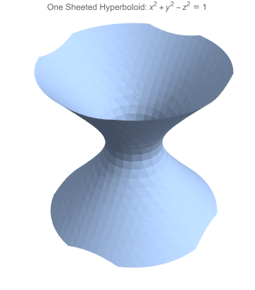
A manifold is a "geometric" object which locally looks like a piece of Euclidean space; by nature it is a continuous object and all its properties are inherently continuous. A first natural class of manifolds are the so called submanifolds of the Euclidean space, for example:
◼
objects described by a number of equation with suitable genericity properties
Region[ImplicitRegion[x^2+y^2-z^2==1,{x,y,z}],PlotRange{{-3,3},{-3,3},{-3,3}},PlotLabelStringJoin[{"One Sheeted Hyperboloid: ",ToString[x^2+y^2-z^2==1,TraditionalForm]}]]
Out[]=
◼
objects described as images of a map from a lower dimensional space
Column[{Style["A Piece of the One Sheeted Hyperboloid from Before Parametrized on a Square",Black],GraphicsRow[{Region@Style[Rectangle[{-1,-1},{1,1}],Orange],Graphics[{Arrowheads[.2],Arrow[BezierCurve[{{0,1},{1,3},{3,3}}]]}],ParametricPlot3D[{x,Sqrt[1-x^2+z^2],z},{x,z}∈Rectangle[{-1,-1},{1,1}],AxesFalse,BoxedFalse,BoxRatios{1,1,1},ViewPoint{.45,.45,.55},Mesh5]},Spacings{{5,5,-5},-5}]},AlignmentCenter]
Out[]=
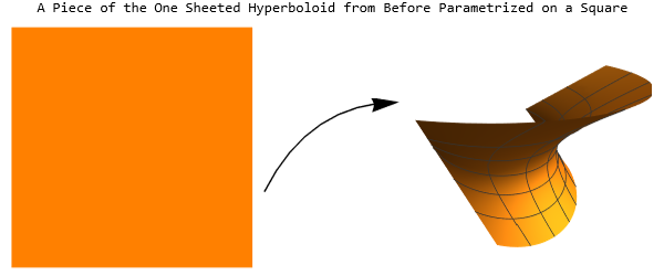
On a manifold, we have a well defined concepts of volume (or area, if the manifold is 2-dimensional as in the previous examples) and of distance between points, which is not the distance in the ambient space (the 3-dimensional space in the first example), or in the parameter space (the rectangle in the second example), but it is the shortest curve that joins two given point and stays always on the manifold. Such curves are called geodesics.
If we pick one point P on a manifold and consider all the points at geodesic distance less than ρ, we obtain what is called a geodesic ball of radius ρ: B(P,ρ). When the radius goes to zero, the volume of such a ball is comparable with the standard euclidean volume of the sphere (which goes as a constant times , if the manifold is n-dimensional); however, the two volumes are not identical and their discrepancy measures what is called (scalar) curvature at P.
n
ρ
Summary and Results
Summary and Results
In a computational setting, we are rarely so lucky to have an explicit equation or a nice parametrization as in the examples before. At times, of a given manifold, we only know a bunch of points, maybe as many as we want, but finitely many.
In order to understand what can be inferred from a discrete sample of points about the geometry of the manifold, we will simulate a random process that generates points according to the volume density of the manifold in a given parameter space. We will then try to give to these points a graph structure, based either on the local distances between them or on the local expected connectivity of a graph lying on a k-dimensional manifold (in terms of the average degree of a vertex); in this way, we have a notion of distance between such points which is not the Euclidean one and hopefully is linked to the geometry of the manifold.
However, our attempts at computing the limiting behavior of the volume, in the small and in the large, will show that the estimator for curvature is too sensitive to changes in the parameters that we use to construct the graph and, even if it can be calculated, it has close to no relationship with the geometry of the underlying manifold.
Poisson Point Processes
The main tool we will be using to generate points that are uniformly distributed on our manifold is the inhomogeneous Poisson point process, which produces independent draws from a given distribution.
We set up the parameter space dimension (n), the embedding space dimension (k), the parametrization function (u) and the parameter region (ℛ) given by our second example from before (we just exchange z and y for convenience) and we proceed to compute a bunch of auxiliary functions and quantities, like the area or ℛ or the area of the piece of manifold parametrized by u over ℛ, which we will call M.
We set up the parameter space dimension (n), the embedding space dimension (k), the parametrization function (u) and the parameter region (ℛ) given by our second example from before (we just exchange z and y for convenience) and we proceed to compute a bunch of auxiliary functions and quantities, like the area or ℛ or the area of the piece of manifold parametrized by u over ℛ, which we will call M.
In[]:=
k=3;n=2;ℛ=Rectangle[{-1,-1},{1,1}];uservars={x,y};(*variablesusedtodescribeuandanysubregionofℛasanImplicitRegion*)u[x_,y_]:={x,y,Sqrt[1-x^2+y^2]};
We create a compiled version of u, compute the volume density of u on ℛ, create a "callable" version of such volume density to be used in our inhomogeneous Poisson point process later on.
In[]:=
variables=Table[Unique["x"],{n}];cu=Compile@@{{#,_Real}&/@#,u@@#,RuntimeOptions"Speed",RuntimeAttributes{Listable},ParallelizationTrue,CompilationOptions{"InlineExternalDefinitions"True}}&[variables];descrℛ=(#[[1]]/.Thread[#[[2]]variables])&[RegionConvert[ℛ,"Implicit"]];canonicalbasis=Table[Table[Boole[i==j],{i,1,n}],{j,1,n}];volmeasureM[vars_List]:=FullSimplify[Norm[Minors[Function[p,(Derivative@@p)[u]@@vars]/@canonicalbasis,n]],vars∈ℛ]callvolmeasureM=Function[#,Evaluate@volmeasureM[#]]&[variables];
Here, we use the volume density function in the most basic way: its integral over ℛ gives the area of the piece of manifold M (hyperboloid, in our case) which is obtained by computing u on the points of ℛ. By comparison, the area of ℛ is (obviously) just 4.
In[]:=
volM=NIntegrate[callvolmeasureM[Sequence@@variables],variables∈ℛ]volR=RegionMeasure[ℛ,n]
Out[]=
5.55794
Out[]=
4
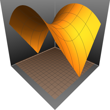
So, the function volmeasureM (or its cognate callvolmeasureM) tells us which parts of ℛ contribute more to the area of M and which parts contribute less: plotting M over ℛ makes it clear that equal parts of ℛ may correspond to pieces of M with different extension.
Show[ParametricPlot3D[u[x,y],{x,y}∈ℛ,AxesFalse,BoxedFalse,BoxRatios{1,1,1},ViewPoint{1,-1,.5},Mesh5],ParametricPlot3D[{x,y,0},{x,-1,1},{y,-1,1},PlotTheme"Marketing",PlotStyleOpacity[0.2]]]
Out[]=
We can now build our Poisson process; however, the number of points we will be getting out of a RandomPointConfiguration call with such a PointProcess will depend by the MeanPointDensity of our point process; in order to be able to draw as many points as we want, we will just have to multiply our function by a suitable correction constant.
In[]:=
myPoissonPointProcess=InhomogeneousPoissonPointProcess[callvolmeasureM,n];correction=1./(volRMeanPointDensity[{myPoissonPointProcess,ℛ}])
Out[]=
0.1844
Random Points Generator
Random Points Generator
We are now ready to define our function to generate random points on ℛ according to the volume density of M. This functions accepts in input the desired number of points and, optionally, the number of configurations of points with such cardinality. Given the random nature of such a process and the mean involved in the definition of the correction from before, the function will return a number of points which is slighlty less than requested.
In[]:=
genRand[numpts_Integer/;numpts>0,nconf_:1]:=Module[{nvM,tPPP},nvM=Function[#,Evaluate[numpts*correction*volmeasureM[#]]]&[variables];tPPP=InhomogeneousPoissonPointProcess[nvM,n];If[nconf==1,Return[RandomPointConfiguration[tPPP,ℛ]["Points"]],Return[RandomPointConfiguration[tPPP,ℛ,nconf]["PointsList"]]]]
As an example, we produce from a thousand to a million points and use Histogram3D to see if their distribution actually approximates the volume distribution function, which we will plot in the end.
In[]:=
GraphicsColumn[Histogram3D[genRand[10^#]]&/@Range[3,6],ImageSize->400]
Out[]=
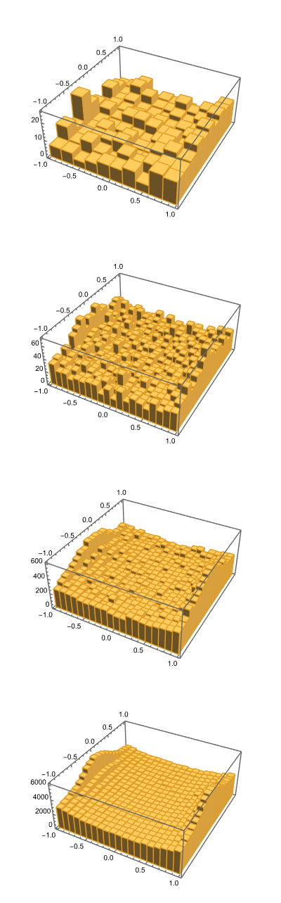
As we can see, when the number of points (1K on the first line of the table, 1M on the last) increases, the approximation of the density is more accurate; this is also reflected in the uniform distribution of the images of such points via u on M. To see this, we compute again random points as before and then we apply to them the function u (or, better, it's compiled version). We go up only to 100K as ListPointPlot3D does not handle well bigger lists; as a comparison, we plot below the manifold M (image of the function u on ℛ).
One can easily see how the distribution is uniform on M, but it is not when projected on ℛ, where, as we know, the point distribute following the law given by the volume density function, which is bigger at some points and smaller at others. This is particularly clear from the first line of plots, with fewer points
Volume Approximation
Volume Approximation
Caution: we will be indistinctly taking about volume and area, because our case-of-study manifold is a surface, but everything we say can be applied to higher dimensional manifolds (with all the obvious drawbacks in terms of execution times and memory usage).
A first test to understand in which sense these points approximate the volume density function is to compute the volume of a subregion in ℛ by counting how many points end up in it; the ratio with the total number of points should converge (as we increase the total number of points) to the ratio between the area of the piece of manifold over the subregion and the area of M.
We define three test subregions in ℛ and group them in the family . Next, we plot them in white over orange.
By integrating the volume density function over these three regions, we obtain the ratio between the volumes of the pieces of manifold parametrized by there three regions and the volume of M.
By using the function genRand and a compiled ad hoc version of Select, we construct a function that generates several configuration of a given number of points and counts how many end up in a given region.
Connecting the Dots
In order to extract some more information from our random points, we try to give them a meaningful graph structure, by connecting with a(n unoriented) edge two points when they are, in some sense, near to each other; we can do that in two ways.
◼
ϵ-Neighbors Graph : (ϵ-graph) we connect two points if their distance is less than a given threshold ϵ.
◼
k-Nearest-Neighbors Graph : (knn-graph) we connect each point with the k nearest points among the others.
Both the previous graphs can be constructed using the function NearestNeighborGraph.
These two choices are, in a way, independent and opposite: the knn-graph will almost always produce something connected and with each vertex of degree exactly k, but it may happen that two fairly distant points are connected because one of them lies in a scarcely populated region.
On the other hand, in a ϵ-graph, all the connected points will always be close, under the ϵ threshold; however, this could result in a high average degree or, if this is kept reasonably low, in a disconnected graph. Moreover, the ϵ-graph is very sensitive with respect to small perturbations of the points, as the following examples show.
On the other hand, in a ϵ-graph, all the connected points will always be close, under the ϵ threshold; however, this could result in a high average degree or, if this is kept reasonably low, in a disconnected graph. Moreover, the ϵ-graph is very sensitive with respect to small perturbations of the points, as the following examples show.
The Perturbed Hexagonal and Square Lattices
The Perturbed Hexagonal and Square Lattices
The following example shows how "fragile" is the behavior of an ϵ-graph when the points are allowed to have "errors" or perturbations.
Already if we use machine precision coordinates, we will fall into rounding errors.
And if we allow for some “noise”, the result is even worse.
With a knn graph we would not have such a problem.
However, who told us that 6 is the right number? If we had come from a square grid, 6 would have produced some awkward results.
From Parametrized Manifolds to Graphs
From Parametrized Manifolds to Graphs
In the Function Repository, one can find two functions to produce graphs from manifolds (ResourceFunction["ExtrinsicCurvedManifoldToGraph"] and ResourceFunction["IntrinsicCurvedManifoldToGraph"] ), which are however limited in use, either by some hypotheses on the nature of the density function we can use or for their prohibitive execution times on large collections of points.
From the documentation, we take one of the examples and increase the number of points.
We propose another function, speeding up the computation in case one is interested only in the graph object per se and getting rid of the restriction on the density function.
This function goes through the steps that we executed in the previous chapter of this notebook, to produce a set of random points which is then fed to the NearestNeighborGraph function.
It is important to notice that the function given as an argument to IntrinsicCurvedManifoldToGraph is already the probability density function from which we want to draw samples; here we pass as an argument the parametrization of the manifold, i.e. the function u, the region ℛ and the list of user variables (used to define u and ℛ). We will test our function on the same number of points, with the same epsilon parameter, on a different function.
To have a visual idea of what is happening, we plot the first three graphs.
As a reference, the manifold we are passing to our new function is the following; we can see a resemblance with the first two graphs, which have a sufficiently low number of vertices to be visualized properly. As a side note, we remark that the image of u is not technically an embedded manifold, because it has a curve of singular points where all the “petals” meet.
Parameters vs Embedding - Epsilon vs KNN
Parameters vs Embedding - Epsilon vs KNN
We plot the first three graphs, which still have a manageable number of vertices and edges - sort of.
The times are comparable, however the same value of ϵ gives slightly different structures:
Another small comparison we have to make is the use of the KNN method to build the graph; we follow the same procedure as before, tabulating the times and plotting the first three graphs.
We can see that there are some peculiar differences with the previous ones, typical of the knn method; moreover, producing less edges, this method is faster.
The remaining comparison, the knn method in the embedding space, would not bring any surprise: applying u will vary small distances in a very similar way, unless we are in points with very different singular values of the Jacobian matrix, which are usually localized phenomena and will not alter the global structure of the graph.
The remaining comparison, the knn method in the embedding space, would not bring any surprise: applying u will vary small distances in a very similar way, unless we are in points with very different singular values of the Jacobian matrix, which are usually localized phenomena and will not alter the global structure of the graph.
The Choice of The ϵ
The Choice of The ϵ
It can be easily guessed that choosing some value of ϵ instead of some other will drastically change the appearance of our graph; one important parameter is the connectedness of the graph, another is the average vertex degree. Both are impossible to determine precisely without actually computing the graph. However, we can approximate the latter with a Monte Carlo method.
This function draws num points from the set of points pts and checks how many points have distance ≤epsilon from each of them, to have an estimate of the average vertex degree of the resulting graph for such a value of epsilon.
We check that the estimate is precise enough.
Using this function, we can determine, given the set of points, which values of epsilon will give reasonable results (i.e. losely in the interval [5,20], where the lower end gives a geometrically significant behavior, whereas the upper end will usually guarantee connectedness, even tho this last fact is not obvious, nor certain).
An empirical analysis shows that this function gives, for a given scale of magnitude, an interesting range of values of epsilon.
An empirical analysis shows that this function gives, for a given scale of magnitude, an interesting range of values of epsilon.
We run a couple of tests; the results are always shown so that different rows refer to different scales of magnitude and different columns to different values of ϵ.
We estimate the average vertex degree of the resulting graph, to see that we generally end up in the interval [5,20].
We construct some ϵ-graphs for the 4 largest values of epsilons[a] and check for their connectedness.
Given that in this intervals for ϵ we find graphs either respecting the combinatorial geometry of planar configurations of points or having the fundamental property of being connected, we will use such ranges of values in all the following simulations.
Shrinking Neighborhoods of a Point
Shrinking Neighborhoods of a Point
The other way of studying the asymptotic of the volume of geodesic balls around a point is to fix the radius of the ball and increase the total number of points.
Again, we varied ϵ, in order to observe various geometric behaviors; the output of the function ball gives us a number of informations, from connectedness to average degree. For the time being, we turn our attention to the volumes of the balls.
As can easily be inferred by these graphs, we need more datapoints and more precision, in order to apply meaningfully any fitting technique. We can however try and change the ϵ, using another dataset. The next three plots are from a list of graphs with average vertex degree near 6.
The following are from a list of graph with very high ϵ, so connected and with high average vertex degree. The fact that the points do not go toward the origin is due to the high number of neighbors of each point, which is non-negligible with respect to the total number of points.
Final Remarks
We have investigated the process of creating a graph from random points on a manifold, highlighting the good properties of approximation of the volume in relation with the number of points in our sample, but also in relation with the parameters employed to create the graph. We want to mention three outcomes of our investigation:
1
.The volume approximation is consistent and increases with the number of points, only slightly influenced by singularities, pinching of curvature and other phenomena.
2
.The estimation of dimension from the growth of the volumes of geodesic balls has a very slow convergence (if it converges), but it seems robust against variations of the parameters of the construction (ϵ, k).
3
.The increasing balls volumes and the shrinking neighborhoods volumes are too sensitive to variations in the parameters to give reliable informations on second order corrections, like scalar curvature: actually, it makes sense that varying ϵ may result in a variation of the scalar curvature of the graph, as it gets more and more different from the geometric structure of the manifold.
Features that would be nice to have
Features that would be nice to have
◼
What is missing here is a way to compute geodesic distances on the manifold, in order to compare the results about graph-geodesic balls to the behavior of the Riemannian geodesic balls on the underlying manifold.
◼
Estimates on the number of datapoints that could give reliable estimates on the second order term of the volume as the neighborhoods approach the point.
◼
An implementation of the Ricci-Ollivier curvature, to be compared with the sectorial growth of volumes (as in the Riemannian case).