In[]:=
dtpts1a={{0,7.81},{7,11.00},{14,11.8},{15.38,11.875},{21,11.6},{28,10.9},{35,10.0},{42,9.11},{49,8.22},{56,7.38},{63,6.62},{70,5.92},{77,5.30},{84,4.74},{91,4.24},{98,3.79},{105,3.38},{112,3.02},{119,2.70}};(*RutherfordB,ProbableCure*)dtpts1b={{15.38,11.875},{21,11.6},{28,10.9},{35,10.0},{42,9.11},{49,8.22},{56,7.38},{63,6.62},{70,5.92},{77,5.30},{84,4.74},{91,4.24},{98,3.79},{105,3.38},{112,3.02},{119,2.70}};(*RutherfordB,ProbableCurefrommaxpointoutto120days*)dtpts1c={{10,11.7},{17,12.4},{24,9.91},{31,9.78},{38,10.1},{45,8.07},{52,7.80},{59,7.80},{66,6.17},{73,5.80},{80,5.59},{87,4.23},{94,3.78},{101,3.43},{108,2.26},{115,1.75}};(*DmpOsc*)dtpts1d={{0.0,10.8},{10,21.9},{20,50.2},{30,64.7},{40,60.4},{50,49.8},{60,44.4},{70,46.1},{80,50.1},{90,52.1},{100,51.4}};(*N049.9,Pf10.9,Pk-38.7k10.033,k20.105,c10.528,c24.12*)dtplt1a=ListPlot[dtpts1a,Frame->True,GridLines->Automatic,PlotRange->{{0,120},{0,15}},ImageSize->{575,366},Joined->True,Mesh->All,PlotStyle->{RGBColor[0,0,1],AbsolutePointSize[10]},AspectRatio->2/π,FrameLabel->{Style["Time (days)",Bold,Blue],Style["ProstateAg",Bold,Blue]},LabelStyle->Directive[Blue,Large]];dtplt1b=ListPlot[dtpts1b,Frame->True,GridLines->Automatic,PlotRange->{{0,120},{0,15}},ImageSize->{575,366},Joined->True,Mesh->All,PlotStyle->{RGBColor[0,0,1],AbsolutePointSize[10]},AspectRatio->2/π,FrameLabel->{Style["Time (days)",Bold,Blue],Style["ProstateAg",Bold,Blue]},LabelStyle->Directive[Blue,Large]];dtplt1c=ListPlot[dtpts1c,Frame->True,GridLines->Automatic,PlotRange->{{0,120},{0,15}},ImageSize->{575,366},Joined->True,Mesh->All,PlotStyle->{RGBColor[0,1,1],AbsolutePointSize[10]},AspectRatio->2/π,FrameLabel->{Style["Time (days)",Bold,Blue],Style["ProstateAg",Bold,Blue]},LabelStyle->Directive[Blue,Large]];dtplt1d=ListPlot[dtpts1d,Frame->True,GridLines->Automatic,PlotRange->{{0,120},{0,15}},ImageSize->{575,366},Joined->True,Mesh->All,PlotStyle->{RGBColor[0,0,1],AbsolutePointSize[10]},AspectRatio->2/π,FrameLabel->{Style["Time (days)",Bold,Blue],Style["ProstateAg",Bold,Blue]},LabelStyle->Directive[Blue,Large]];
In[]:=
E2aDampedOscillator:=N0+(Pf×((Exp[-(k1×t)])×((c1×Cos[k2×(t-Pk)]))));E2aDOsc[N0_,Pf_,Pk_,k1_,c1_,k2_]:=N0+(Pf×((Exp[-(k1×(t-Pk))])×((c1×Cos[k2×(t-Pk)]))));gRa[t_,r_,N0_,Pf_,Pk_,k1_,c1_,k2_]:=((t×r)+(E2aDOsc[N0,Pf,Pk,k1,c1,k2]));
In[]:=
Clear[t,E2DOsc,gR,r,N0,Pf,Pk,k1,c1,k2]E2DOsc[N0_,Pf_,Pk_,k1_,c1_,k2_]:=N0+(Pf×((Exp[-(k1×(t-Pk))])×((c1×Cos[k2×(t-Pk)]))));gR[t_,r_,N0_,Pf_,Pk_,k1_,c1_,k2_]:=((t×r)+(E2DOsc[N0,Pf,Pk,k1,c1,k2]));
In[]:=
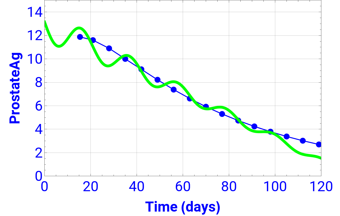
Manipulate[Show[Plot[gR[t,r,N0,Pf,Pk,k1,c1,k2],{t,0.0,120.0},Frame->True,GridLines->Automatic,AxesOrigin->{0.0,0.0},PlotRange->{{0,120},{0,15}},ImageSize->{575,366},PlotStyle->{RGBColor[0,1,0],Thickness[0.01]},AspectRatio->2.0/π,FrameLabel->{Style["Time (days)",Bold,Blue],Style["ProstateAg",Bold,Blue]},LabelStyle->Directive[Blue,Large]],dtplt1b,dtplt1c],{{N0,13.0,Style["Initial (N0)",Blue,Bold,Medium]},0.0,20.0,0.00010,ControlType->Slider,ImageSize->Medium,DefaultBaseStyle->{Blue,Bold,Medium},Appearance->"Labeled"},{{Pf,1.0,Style["Power Factor (Pf)",Blue,Bold,Medium]},-10.0,10.0,0.00010,ControlType->Slider,ImageSize->Medium,DefaultBaseStyle->{Blue,Bold,Medium},Appearance->"Labeled"},{{Pk,16.0,Style["Peak Location (Pk)",Blue,Bold,Medium]},0.0,25.0,0.00010,ControlType->Slider,ImageSize->Medium,DefaultBaseStyle->{Blue,Bold,Medium},Appearance->"Labeled"},{{k1,0.016,Style["Damping (k1)",Blue,Bold,Medium]},-0.10,0.10,0.00010,ControlType->Slider,ImageSize->Medium,DefaultBaseStyle->{Blue,Bold,Medium},Appearance->"Labeled"},{{c1,1.5,Style["Cos (c1)",Blue,Bold,Medium]},0.0,5.0,0.00010,ControlType->Slider,ImageSize->Medium,DefaultBaseStyle->{Blue,Bold,Medium},Appearance->"Labeled"},{{k2,0.3,Style["Period (k2)",Blue,Bold,Medium]},0.010,0.50,0.00010,ControlType->Slider,ImageSize->Medium,DefaultBaseStyle->{Blue,Bold,Medium},Appearance->"Labeled"},{{r,-0.0975,Style["Rotate (r)",Blue,Bold,Medium]},-5,5,0.00010,ControlType->Slider,ImageSize->Medium,DefaultBaseStyle->{Blue,Bold,Medium},Appearance->"Labeled"},ControlPlacement->Top,Paneled->True,ImageMargins->0]
Out[]=

In[]:=
KinetE2DO=NonlinearModelFit[dtpts1c,gR[t,r,N0,Pf,Pk,k1,c1,k2],{{r,-0.0975},{N0,13},{Pf,1.0},{Pk,16},{k1,0.016},{c1,1.5},{k2,0.3}},t,Method->"Automatic"]
Out[]=
FittedModel
In[]:=
Normal[KinetE2DO]
Out[]=
12.9925-0.0974099t+1.14724Cos[0.300232(-16.0534+t)]
-0.0156507(-16.0534+t)
In[]:=
KinetEBR["BestFitParameters"]
Out[]=
KinetEBR[BestFitParameters]
In[]:=
KinetE2DO["ParameterErrors"]
Out[]=
{0.000121521,0.00859839,0.00628255,0.0313888,0.000339868,0.0055232,0.000298436}
In[]:=
KinetE2DO["ParameterTable"]
Out[]=
Estimate | Standard Error | t-Statistic | P-Value | |
r | -0.0974099 | 0.000121521 | -801.589 | 3.72634× -23 10 |
N0 | 12.9925 | 0.00859839 | 1511.04 | 1.23985× -25 10 |
Pf | 1.00428 | 0.00628255 | 159.852 | 7.4608× -17 10 |
Pk | 16.0534 | 0.0313888 | 511.439 | 2.12652× -21 10 |
k1 | 0.0156507 | 0.000339868 | 46.0494 | 5.37441× -12 10 |
c1 | 1.14235 | 0.0055232 | 206.828 | 7.34551× -18 10 |
k2 | 0.300232 | 0.000298436 | 1006.02 | 4.82386× -24 10 |
In[]:=
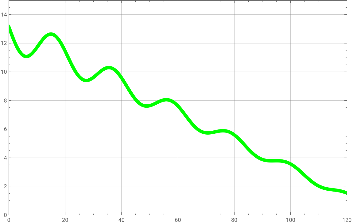
KinetE2DOscMdl=Plot[{KinetE2DO[t]},{t,0,120},PlotRange->{{0,120},{0.0,15.0}},Frame->True,GridLines->Automatic,ImageSize->{575,366},PlotStyle->{Green,Thickness[0.01]},AspectRatio->2/π]
Out[]=
In[]:=
Show[dtplt1b,KinetE2DOscMdl]
Out[]=