ABSTRACT (original article): Many chemical engineering programs teach gas permeation because of its important applications in the oil and gas industry. In fact, it is considered a good replacement for classical separation techniques such as cryogenic technologies, PSA, physical and chemical absorption etc. Gas permeation module modeling can play an important role in both simulation and design of permeation units. In fact, the simulation allows the prediction of the separation performance of gas permeation modules as well as the selection of optimal operating parameters, stage cut and pressure ratio . On the other hand, the design provides useful data such as the module area. Here, we present the theoretical background of this unit operation, and the modeling of a single-stage gas permeation module used to separate multicomponent gas mixtures for the following flow patterns: (1) perfect mixing, (2) one-side mixing, (3) cross flow, (4) co-current flow, (4) counter-current flow. Our numerical simulation methodology is based on Chebyshev orthogonal collocation and arc-length continuation techniques. We apply the proposed methodology to two industrially important systems, which are described in reference (Shindo et al. in Sep Sci Technol 20:445–459, 1985. https:// doi. org/ 10. 1080/ 01496 39850 80606 92): (1) separation of NH3, H2, and N2 gaseous mixture by means of a polyethylene membrane. Such a gas mixture arises in the Haber process. (2) Separation of H2, CH4, CO, N2, and CO2 mixture through a microporous glass membrane. This mixture is important in the partial oxidation of fuels with air and in the steam gasification of biomass. Whenever possible, our results are benchmarked against data obtained from the open literature or predicted using the software Aspen-Plus®. Furthermore, we performed sensitivity analyses where we vary either the stage cut or the pressure ratio in order to investigate the effect of these parameters on both the permeate and retentate compositions as well as on the surface area of the permeation module. Finally, we provide useful tips and computer coding to readers who wish to investigate similar gas permeation problems using our new methodology. CITATION (original article): H. Binous, U. Zahid and A. Bellagi, Modeling for Multi-component Gas Permeation with Orthogonal Collocation and Arc-Length Continuation, Chemistry Africa (2024). DOI: https://doi.org/10.1007/s42250-024-01167-y
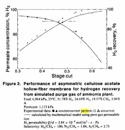
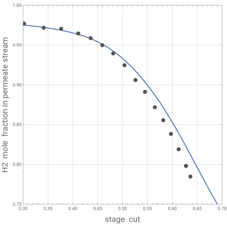
Hydrogen recovery from purge gas of ammonia plant is important. Pan compared model and experimental data for hydrogen percent recovery and hydrogen mole fraction in the permeate stream at various values of stage cut (see Fig. 2 of Ref. 1). Here, we reproduce Fig. 2 of Ref. 1 using a counter-current gas permeation module and the methodology described in detail in Ref. 2.
In[]:=
Out[]=
{xA[1]0.500575,xB[1]0.255751,xC[1]0.202724,xA[2]0.500682,xB[2]0.255696,xC[2]0.20268,xA[3]0.501001,xB[3]0.255532,xC[3]0.20255,xA[4]0.501523,xB[4]0.255263,xC[4]0.202337,xA[5]0.502236,xB[5]0.254897,xC[5]0.202046,xA[6]0.503121,xB[6]0.254442,xC[6]0.201685,xA[7]0.504156,xB[7]0.25391,xC[7]0.201263,xA[8]0.505315,xB[8]0.253315,xC[8]0.20079,xA[9]0.506569,xB[9]0.252671,xC[9]0.200279,xA[10]0.507887,xB[10]0.251993,xC[10]0.199742,xA[11]0.509235,xB[11]0.2513,xC[11]0.199192,xA[12]0.510582,xB[12]0.250609,xC[12]0.198643,xA[13]0.511893,xB[13]0.249935,xC[13]0.198108,xA[14]0.513136,xB[14]0.249296,xC[14]0.197601,xA[15]0.514282,xB[15]0.248708,xC[15]0.197134,xA[16]0.515302,xB[16]0.248183,xC[16]0.196718,xA[17]0.516172,xB[17]0.247736,xC[17]0.196364,xA[18]0.516871,xB[18]0.247377,xC[18]0.196079,xA[19]0.517383,xB[19]0.247114,xC[19]0.19587,xA[20]0.517695,xB[20]0.246954,xC[20]0.195743,yA[2]0.983438,yB[2]0.00760996,yC[2]0.00580118,yA[3]0.983451,yB[3]0.0076041,yC[3]0.00579671,yA[4]0.983471,yB[4]0.00759451,yC[4]0.0057894,yA[5]0.9835,yB[5]0.00758145,yC[5]0.00577943,yA[6]0.983535,yB[6]0.00756525,yC[6]0.00576708,yA[7]0.983576,yB[7]0.00754636,yC[7]0.00575267,yA[8]0.983622,yB[8]0.00752526,yC[8]0.00573658,yA[9]0.983671,yB[9]0.0075025,yC[9]0.00571922,yA[10]0.983723,yB[10]0.00747865,yC[10]0.00570103,yA[11]0.983775,yB[11]0.00745432,yC[11]0.00568247,yA[12]0.983828,yB[12]0.0074301,yC[12]0.00566401,yA[13]0.983879,yB[13]0.0074066,yC[13]0.00564608,yA[14]0.983927,yB[14]0.00738437,yC[14]0.00562913,yA[15]0.983971,yB[15]0.00736395,yC[15]0.00561355,yA[16]0.984011,yB[16]0.00734581,yC[16]0.00559972,yA[17]0.984044,yB[17]0.00733037,yC[17]0.00558794,yA[18]0.984071,yB[18]0.00731798,yC[18]0.00557849,yA[19]0.984091,yB[19]0.00730893,yC[19]0.00557159,yA[20]0.984103,yB[20]0.00730341,yC[20]0.00556738,yA[21]0.984107,yB[21]0.00730156,yC[21]0.00556597,q[2]0.96459,q[3]0.965228,q[4]0.966274,q[5]0.967705,q[6]0.969487,q[7]0.97158,q[8]0.973933,q[9]0.976492,q[10]0.979195,q[11]0.981976,q[12]0.984768,q[13]0.987501,q[14]0.990107,q[15]0.99252,q[16]0.994678,q[17]0.996525,q[18]0.998015,q[19]0.999108,q[20]0.999776,theta0.035624,0.983434,0.00761193,0.00580268,0.0031517}
y
PAi
y
PBi
y
PCi
y
PDi
In[]:=
xA[Np+1]=.;xB[Np+1]=.;xC[Np+1]=.;q[Np+1]=.;q[1]=.;yA[1]=.;yB[1]=.;yC[1]=.;xA[Np+1][s_]:=;xB[Np+1][s_]:=;yA[1][s_]:=[s];yB[1][s_]:=[s];xC[Np+1][s_]:=;yC[1][s_]:=[s];q[Np+1][s_]:=;q[1][s_]:=(1-theta[s]);init=Join[Flatten[Table[{xA[i][0](xA[i]/.sol),yA[i][0](yA[i]/.sol),xC[i][0](xC[i]/.sol),yC[i][0](yC[i]/.sol),xB[i][0](xB[i]/.sol),yB[i][0](yB[i]/.sol)},{i,2,Np}],1],Flatten[Table[q[i][0](q[i]/.sol),{i,2,Np}],1],{theta[0](theta/.sol),[0](/.sol),st[0]0.001,yA[1][0](/.sol),yB[1][0](/.sol),yC[1][0](/.sol),yA[Np+1][0](yA[Np+1]/.sol),yB[Np+1][0](yB[Np+1]/.sol),yC[Np+1][0](yC[Np+1]/.sol),xA[1][0](xA[1]/.sol),xC[1][0](xC[1]/.sol),xB[1][0](xB[1]/.sol)}];initdev=Join[Flatten[Table[{xA[i]'[0]-0.1,yA[i]'[0]-0.1,xB[i]'[0]0.1,yB[i]'[0]0.1,xC[i]'[0]-0.1,yC[i]'[0]-0.1},{i,2,Np}],1],Flatten[Table[{q[i]'[0]-0.1},{i,2,Np}],1],{theta'[0]0.1,st'[0]0.1,xA[1]'[0]-0.1,xC[1]'[0]-0.1,xB[1]'[0]0.1,'[0]0.1,'[0]0.1,'[0]0.1,'[0]0.1,yA[Np+1]'[0]-0.1,yB[Np+1]'[0]-0.1,yC[Np+1]'[0]-0.1}];aux=Sum[xA[i]'[s]^2+yA[i]'[s]^2+xB[i]'[s]^2+yB[i]'[s]^2+xC[i]'[s]^2+yC[i]'[s]^2,{i,1,Np}]+Sum[q[i]'[s]^2,{i,2,Np}]+theta'[s]^2+st'[s]^2+'[s]^2+'[s]^2+'[s]^2+'[s]^2+yA[21]'[s]^2+yB[21]'[s]^2+yC[21]'[s]^21;unknown1=Join[Flatten[Table[{xA[i],yA[i],xB[i],yB[i],xC[i],yC[i]},{i,2,Np}],1],Flatten[Table[q[i],{i,2,Np}],1],{,,,,theta,st,yA[Np+1],yB[Np+1],yC[Np+1],xA[1],xB[1],xC[1]}];
x
fA
x
fB
y
PAi
y
PBi
x
fC
y
PCi
q
f
q
f
y
PDi
y
PDi
y
PAi
y
PBi
y
PCi
y
PAi
y
PBi
y
PCi
y
PDi
y
PAi
y
PBi
y
PDi
y
PCi
y
PAi
y
PBi
y
PCi
y
PDi
In[]:=
In[]:=
SYS=Join[sys/.functions,{aux},init,initdev];SOL=Quiet@NDSolve[SYS,unknown1,{s,-1000,1000},AccuracyGoal5];
Check material balance for H2
In[]:=
solA=First@NSolve[theta[s]yAP+(1-theta[s])xA[1][s]0.5178,yAP]
Out[]=
yAP
0.5178-1.(1.-1.theta[s])xA[1][s]
theta[s]
In[]:=
TableForm[Table[{yAP/.solA,yA[Np+1][s]}/.SOL[[1]],{s,-5,65,5}]]
Out[]//TableForm=
0.879462 | 0.879463 |
0.984107 | 0.984107 |
0.993703 | 0.993703 |
0.995747 | 0.995745 |
0.996697 | 0.996696 |
0.997263 | 0.997264 |
0.997646 | 0.997649 |
0.997923 | 0.997928 |
0.998136 | 0.998136 |
0.998305 | 0.998304 |
0.998442 | 0.998442 |
0.998557 | 0.998557 |
0.998654 | 0.998653 |
0.998737 | 0.998737 |
0.99881 | 0.99881 |
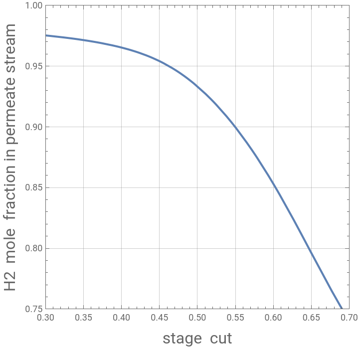
Mole fraction of H2 in the permeate stream versus stage cut
In[]:=
pA=ParametricPlot[Evaluate[{theta[s],yA[Np+1][s]}/.SOL[[1]]],{s,-8.9,65},PlotRange{{0.3,0.7},{0.75,1.0}},FrameTrue,GridLinesAutomatic,AspectRatio1,PlotStyleThick,FrameTrue,FrameLabel{Style["stage cut",16],Style["H2 mole fraction in permeate stream",16]}]
Out[]=
Digitized data of mole fraction of H2 in the permeate stream obtained from Fig. 2 of Ref. 1
In[]:=
digitizeddatafig2pan={{0.302067162349865,0.97686902524716},{0.34152027671106,0.971792357763433},{0.376566712966745,0.970430590734537},{0.410915924503635,0.96458861018057},{0.435776343383174,0.958711223683852},{0.459198736280197,0.949843396791677},{0.503908271372933,0.924637089086799},{0.545028188577498,0.891208432061443},{0.564877304790696,0.871879510853283},{0.481172209058474,0.939477626167715},{0.525941661900482,0.906062586812648},{0.581785004221477,0.855524688836234},{0.597238336465397,0.838418171419233},{0.612708009913663,0.819072909006727},{0.627458670370672,0.798232426396492},{0.627458670370672,0.798232426396492},{0.636315603126617,0.784832638832148}};
In[]:=
p2=ListPlot[digitizeddatafig2pan,PlotStyle{PointSize[0.02],Darker@Gray}];
Comparison between our calculation and digitized data from Fig. 2 of Ref. 1
In[]:=
Show[pA,p2,ImageSize450{1,1}]
Out[]=
Percent recovery of H2 in the permeate stream versus stage cut
Digitized data for percent recovery of H2 obtained from Fig. 2 of Ref. 1
Comparison between our calculation and digitized data from Fig. 2 of Ref. 1
References
References
[1] Pan, C.Y. (1986), Gas separation by high-flux, asymmetric hollow-fiber membrane. AIChE J., 32: 2020-2027. https://doi.org/10.1002/aic.690321212
[2] H . Binous, U . Zahid and A . Bellagi, Modeling for Multi - component Gas Permeation with Orthogonal Collocation and Arc - Length Continuation, Chemistry Africa (2024) . https://doi .org/10.1007/s42250-024-01167-y
[2] H . Binous, U . Zahid and A . Bellagi, Modeling for Multi - component Gas Permeation with Orthogonal Collocation and Arc - Length Continuation, Chemistry Africa (2024) . https://doi .org/10.1007/s42250-024-01167-y
CITE THIS NOTEBOOK
CITE THIS NOTEBOOK
Hydrogen recovery form ammonia plant purge stream
by Housam Binous and Ahmed Bellagi
Wolfram Community, STAFF PICKS, December 29, 2024
https://community.wolfram.com/groups/-/m/t/3346371
by Housam Binous and Ahmed Bellagi
Wolfram Community, STAFF PICKS, December 29, 2024
https://community.wolfram.com/groups/-/m/t/3346371