Abstract
Abstract
The school method for numerically solving physics problems is to integrate the Euler-Lagrange equation (https://en.wikipedia.org/wiki/Euler%E2%80%93Lagrange_equation). In this method, one
1
.writes a Lagrangian from the physics for the system
2
.symbolically applies the variational principle, e.g., Hamilton’s Principle, to derive the Euler-Lagrange equation
3
.discretizes time or its surrogate independent variable, e.g., proper time
4
.integrates the discretized equation with respect to that discretized variable given some initial conditions
The school method has many numerical hazards and has spawned an enormous literature.
One of the most interesting alternatives is to discretize the Lagrangian before applying the variational principle, producing an iterable or recursive algebraic equation that can be stepped explicitly or implicitly. There is a growing literature on this alternative. One early reference by Kobilarov and Marsden explains it well and is cited and tested in this note on a foundational case: the undamped simple harmonic oscillator. This example illustrates and supports the un-numbered equations in Section II of the referenced paper.
Undamped Simple Harmonic Oscillator
Undamped Simple Harmonic Oscillator
In[]:=
ClearAll[L,V,Ld];
Analytical Solution
Analytical Solution
Potential energy.
In[]:=
V[q_]:=κ
1
2
2
q
Lagrangian.
In[]:=
L[q_,v_,t_]:=m-V[q]
1
2
2
v
Second term of the Euler-Lagrange equations: a total derivative of the partial derivative of the Lagrangian with respect to generalized velocity , which entails a derivative of mass with respect to time via the chain rule. We insert an explicit correction for constant mass by setting the derivative of mass with respect to time to 0. Non-constant mass would be useful for, say, the rocket equation, but is not pertinent here.
L
v
In[]:=
Dt[D[L[q,v,t],v],t]/.{Dt[m,t]->0}
Out[]=
mDt[v,t]
First term of the Euler-Lagrange equations. No explicit assumption of constant spring-force coefficient is necessary because this term is just a partial derivative of with respect to and does not entail the chain rule.
κ
L
q
In[]:=
D[L[q,v,t],q]
Out[]=
-qκ
The Euler-Lagrange equations. By inspection, they are equal to the naive Newtonian equations of motion for this undamped oscillator.
In[]:=
deqn=((D[L[q,v,t],q]-(Dt[D[L[q,v,t],v],t]/.{Dt[m,t]->0}/.{v->Dt[q,t]})/.{q->x[t]})==0)
Out[]=
-κx[t]-m[t]0
′′
x
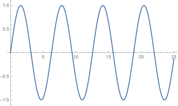
Mathematica easily solves them. We pick the solution, as a function, from the structure returned by Mathematica’s DSolve.
In[]:=
dsoln=(DSolve[deqn,x,t])[[1,1,2]]
Out[]=
Function{t},Cos+Sin
1
t
κ
m
2
t
κ
m
In[]:=
Plot[dsoln[t]/.{κ->1,m->1,C[2]->1,C[1]->0},{t,0,25}]
Out[]=
Discrete Solution
Discrete Solution
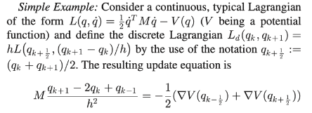
Quadrature of the discrete Lagrangian, which actually has units of action, i.e., energy times time, according to the third, unnumbered equation on page 643 of the reference.
In[]:=
discreteEqn=m==-D[V[q],q]/.q->+D[V[q],q]/.q->
q[k+1]-2q[k]+q[k-1]
2
h
1
2
q[k-1]+q[k]
2
q[k]+q[k+1]
2
Out[]=
m(q[-1+k]-2q[k]+q[1+k])
2
h
1
2
1
2
1
2
Algebraic solution of the discrete equation for time step given solutions for time steps and . Do not confuse time step with spring constant .
k+1
k-1
k
k
κ
In[]:=
discreteSoln=(Solve[discreteEqn,q[1+k]]//FullSimplify)[[1,1,2]]
Out[]=
-q[-1+k]+
2(4m-κ)q[k]
2
h
4m+κ
2
h
For integration and plotting, manually substitute the discrete solution (the expression (discreteSoln...) does not work for unknown reasons)
In[]:=
(discreteSoln/.{κ->1,m->1})
Out[]=
-q[-1+k]+
2(4-)q[k]
2
h
4+
2
h
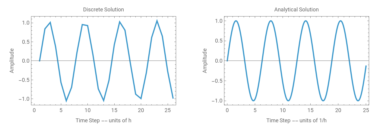
Compare the plot of the analytical solution versus the discrete solution for various choices of the time step, represented by its negative logarithm base 10.
In[]:=
ClearAll[experiment];experiment[timeSteps_,h_]:=Module{k,q,x},q[k_]:=x[[1+k]];x=ConstantArray[0,timeSteps+1];x[[1]]=0;x[[2]]=Sin[h];Fork=1,k<timeSteps,k++,x[[k+2]]=-q[-1+k]+;GraphicsRow[{ListLinePlot[x,Frame->True,FrameLabel->{{"Amplitude",""},{"Time Step -- units of h","Discrete Solution"}}],Plot[dsoln[τ]/.{κ->1,m->1,C[2]->1,C[1]->0},{τ,0,timeStepsh},Frame->True,FrameLabel->{{"Amplitude",""},{"Time Step -- units of 1/h","Analytical Solution"}}]}];Manipulateexperiment25,,{minuslog10h,{0,-1,-2,-3,-4}},SaveDefinitions->True
2(4-)q[k]
2
h
4+
2
h
minuslog10h
10
minuslog10h
10.
Out[]=

Reference
Reference
Marin Kobilarov and Jerrold E. Marsden, Discrete Geometric Optimal Control on Lie Groups, IEEE Transactions on Robotics, Vol. 27, No. 4, August 2011.
CITE THIS NOTEBOOK
CITE THIS NOTEBOOK
Harmonic oscillator via discrete Lagrangian
by Brian Beckman
Wolfram Community, STAFF PICKS, April 19, 2024
https://community.wolfram.com/groups/-/m/t/3161109
by Brian Beckman
Wolfram Community, STAFF PICKS, April 19, 2024
https://community.wolfram.com/groups/-/m/t/3161109